Two-dimensional space
In physics and mathematics, two-dimensional space or bi-dimensional space is a geometric model of the planar projection of the physical universe. The two dimensions are commonly called length and width. Both directions lie in the same plane.
A sequence of n real numbers can be understood as a location in n-dimensional space. When n = 2, the set of all such locations is called two-dimensional space or bi-dimensional space, and usually is thought of as a Euclidean space.
History
Books I through IV and VI of Euclid's Elements dealt with two-dimensional geometry, developing such notions as similarity of shapes, the Pythagorean theorem (Proposition 47), equality of angles and areas, parallelism, the sum of the angles in a triangle, and the three cases in which triangles are "equal" (have the same area), among many other topics.
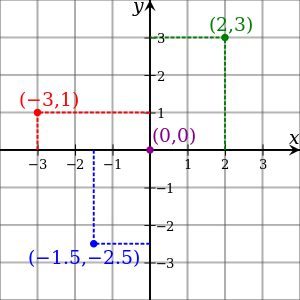
Later, the plane was described in a so-called Cartesian coordinate system, a coordinate system that specifies each point uniquely in a plane by a pair of numerical coordinates, which are the signed distances from the point to two fixed perpendicular directed lines, measured in the same unit of length. Each reference line is called a coordinate axis or just axis of the system, and the point where they meet is its origin, usually at ordered pair (0, 0). The coordinates can also be defined as the positions of the perpendicular projections of the point onto the two axes, expressed as signed distances from the origin.
The idea of this system was developed in 1637 in writings by Descartes and independently by Pierre de Fermat, although Fermat also worked in three dimensions, and did not publish the discovery.[1] Both authors used a single axis in their treatments and have a variable length measured in reference to this axis. The concept of using a pair of axes was introduced later, after Descartes' La Géométrie was translated into Latin in 1649 by Frans van Schooten and his students. These commentators introduced several concepts while trying to clarify the ideas contained in Descartes' work.[2]
Later, the plane was thought of as a field, where any two points could be multiplied and, except for 0, divided. This was known as the complex plane. The complex plane is sometimes called the Argand plane because it is used in Argand diagrams. These are named after Jean-Robert Argand (1768–1822), although they were first described by Norwegian-Danish land surveyor and mathematician Caspar Wessel (1745–1818).[3] Argand diagrams are frequently used to plot the positions of the poles and zeroes of a function in the complex plane.
In geometry
Coordinate systems
In mathematics, analytic geometry (also called Cartesian geometry) describes every point in two-dimensional space by means of two coordinates. Two perpendicular coordinate axes are given which cross each other at the origin. They are usually labeled x and y. Relative to these axes, the position of any point in two-dimensional space is given by an ordered pair of real numbers, each number giving the distance of that point from the origin measured along the given axis, which is equal to the distance of that point from the other axis.
Another widely used coordinate system is the polar coordinate system, which specifies a point in terms of its distance from the origin and its angle relative to a rightward reference ray.


Polytopes
In two dimensions, there are infinitely many polytopes: the polygons. The first few regular ones are shown below:
Convex
The Schläfli symbol {p} represents a regular p-gon.
| Name | Triangle (2-simplex) |
Square (2-orthoplex) (2-cube) |
Pentagon | Hexagon | Heptagon | Octagon | |
|---|---|---|---|---|---|---|---|
| Schläfli | {3} | {4} | {5} | {6} | {7} | {8} | |
| Image |  |
 |
 |
 |
 |
 | |
| Name | Nonagon | Decagon | Hendecagon | Dodecagon | Triskaidecagon | Tetradecagon | |
| Schläfli | {9} | {10} | {11} | {12} | {13} | {14} | |
| Image |  |
 |
 |
 |
 |
 | |
| Name | Pentadecagon | Hexadecagon | Heptadecagon | Octadecagon | Enneadecagon | Icosagon | ...n-gon |
| Schläfli | {15} | {16} | {17} | {18} | {19} | {20} | {n} |
| Image |  |
 |
 |
 |
 |
 |
Degenerate (spherical)
The regular henagon {1} and regular digon {2} can be considered degenerate regular polygons. They can exist nondegenerately in non-Euclidean spaces like on a 2-sphere or a 2-torus.
| Name | Henagon | Digon |
|---|---|---|
| Schläfli | {1} | {2} |
| Image |  |
 |
Non-convex
There exist infinitely many non-convex regular polytopes in two dimensions, whose Schläfli symbols consist of rational numbers {n/m}. They are called star polygons and share the same vertex arrangements of the convex regular polygons.
In general, for any natural number n, there are n-pointed non-convex regular polygonal stars with Schläfli symbols {n/m} for all m such that m < n/2 (strictly speaking {n/m} = {n/(n − m)}) and m and n are coprime.
| Name | Pentagram | Heptagrams | Octagram | Enneagrams | Decagram | ...n-agrams | ||
|---|---|---|---|---|---|---|---|---|
| Schläfli | {5/2} | {7/2} | {7/3} | {8/3} | {9/2} | {9/4} | {10/3} | {n/m} |
| Image |  |
 |
 |
 |
 |
 |
 |
|
Circle
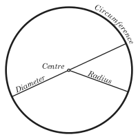
The hypersphere in 2 dimensions is a circle, sometimes called a 1-sphere (S1) because it is a one-dimensional manifold. In a Euclidean plane, it has the length 2πr and the area of its interior is

where is the radius.

Other shapes
There are an infinitude of other curved shapes in two dimensions, notably including the conic sections: the ellipse, the parabola, and the hyperbola.
In linear algebra
Another mathematical way of viewing two-dimensional space is found in linear algebra, where the idea of independence is crucial. The plane has two dimensions because the length of a rectangle is independent of its width. In the technical language of linear algebra, the plane is two-dimensional because every point in the plane can be described by a linear combination of two independent vectors.
Dot product, angle, and length
The dot product of two vectors A = [A1, A2] and B = [B1, B2] is defined as:[4]

A vector can be pictured as an arrow. Its magnitude is its length, and its direction is the direction the arrow points. The magnitude of a vector A is denoted by . In this viewpoint, the dot product of two Euclidean vectors A and B is defined by[5]


where θ is the angle between A and B.
The dot product of a vector A by itself is

which gives

the formula for the Euclidean length of the vector.
In calculus
Gradient
In a rectangular coordinate system, the gradient is given by

Line integrals and double integrals
For some scalar field f : U ⊆ R2 → R, the line integral along a piecewise smooth curve C ⊂ U is defined as

where r: [a, b] → C is an arbitrary bijective parametrization of the curve C such that r(a) and r(b) give the endpoints of C and .

For a vector field F : U ⊆ R2 → R2, the line integral along a piecewise smooth curve C ⊂ U, in the direction of r, is defined as

where · is the dot product and r: [a, b] → C is a bijective parametrization of the curve C such that r(a) and r(b) give the endpoints of C.
A double integral refers to an integral within a region D in R2 of a function and is usually written as:


Fundamental theorem of line integrals
The fundamental theorem of line integrals, says that a line integral through a gradient field can be evaluated by evaluating the original scalar field at the endpoints of the curve.
Let . Then

![\varphi \left(\mathbf {q} \right)-\varphi \left(\mathbf {p} \right)=\int _{\gamma [\mathbf {p} ,\,\mathbf {q} ]}\nabla \varphi (\mathbf {r} )\cdot d\mathbf {r} .](../I/m/b27cdd0377931a70cbb0635e37781a42e7fe33f9.svg)
Green's theorem
Let C be a positively oriented, piecewise smooth, simple closed curve in a plane, and let D be the region bounded by C. If L and M are functions of (x, y) defined on an open region containing D and have continuous partial derivatives there, then[6][7]

where the path of integration along C is counterclockwise.
In topology
In topology, the plane is characterized as being the unique contractible 2-manifold.
Its dimension is characterized by the fact that removing a point from the plane leaves a space that is connected, but not simply connected.
In graph theory
In graph theory, a planar graph is a graph that can be embedded in the plane, i.e., it can be drawn on the plane in such a way that its edges intersect only at their endpoints. In other words, it can be drawn in such a way that no edges cross each other.[8] Such a drawing is called a plane graph or planar embedding of the graph. A plane graph can be defined as a planar graph with a mapping from every node to a point on a plane, and from every edge to a plane curve on that plane, such that the extreme points of each curve are the points mapped from its end nodes, and all curves are disjoint except on their extreme points.
References
- ↑ "Analytic geometry". Encyclopædia Britannica (Encyclopædia Britannica Online ed.). 2008.
- ↑ Burton 2011, p. 374
- ↑ Wessel's memoir was presented to the Danish Academy in 1797; Argand's paper was published in 1806. (Whittaker & Watson, 1927, p. 9)
- ↑ S. Lipschutz; M. Lipson (2009). Linear Algebra (Schaum’s Outlines) (4th ed.). McGraw Hill. ISBN 978-0-07-154352-1.
- ↑ M.R. Spiegel; S. Lipschutz; D. Spellman (2009). Vector Analysis (Schaum’s Outlines) (2nd ed.). McGraw Hill. ISBN 978-0-07-161545-7.
- ↑ Mathematical methods for physics and engineering, K.F. Riley, M.P. Hobson, S.J. Bence, Cambridge University Press, 2010, ISBN 978-0-521-86153-3
- ↑ Vector Analysis (2nd Edition), M.R. Spiegel, S. Lipschutz, D. Spellman, Schaum’s Outlines, McGraw Hill (USA), 2009, ISBN 978-0-07-161545-7
- ↑ Trudeau, Richard J. (1993). Introduction to Graph Theory (Corrected, enlarged republication. ed.). New York: Dover Pub. p. 64. ISBN 978-0-486-67870-2. Retrieved 8 August 2012.
Thus a planar graph, when drawn on a flat surface, either has no edge-crossings or can be redrawn without them.
See also
| Dimensional spaces |  | |
|---|---|---|
| Other dimensions | ||
| Polytopes and shapes | ||
| Dimensions by number | ||
Category | ||