Coordinate system
In geometry, a coordinate system is a system which uses one or more numbers, or coordinates, to uniquely determine the position of a point or other geometric element on a manifold such as Euclidean space.[1][2] The order of the coordinates is significant, and they are sometimes identified by their position in an ordered tuple and sometimes by a letter, as in "the x-coordinate". The coordinates are taken to be real numbers in elementary mathematics, but may be complex numbers or elements of a more abstract system such as a commutative ring. The use of a coordinate system allows problems in geometry to be translated into problems about numbers and vice versa; this is the basis of analytic geometry.[3]
Common coordinate systems
Number line
The simplest example of a coordinate system is the identification of points on a line with real numbers using the number line. In this system, an arbitrary point O (the origin) is chosen on a given line. The coordinate of a point P is defined as the signed distance from O to P, where the signed distance is the distance taken as positive or negative depending on which side of the line P lies. Each point is given a unique coordinate and each real number is the coordinate of a unique point.[4]

Cartesian coordinate system
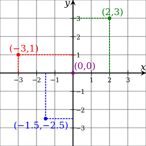
The prototypical example of a coordinate system is the Cartesian coordinate system. In the plane, two perpendicular lines are chosen and the coordinates of a point are taken to be the signed distances to the lines.

In three dimensions, three perpendicular planes are chosen and the three coordinates of a point are the signed distances to each of the planes.[5] This can be generalized to create n coordinates for any point in n-dimensional Euclidean space.
Depending on the direction and order of the coordinate axis the system may be a right-hand or a left-hand system. This is one of many coordinate systems.
Polar coordinate system
Another common coordinate system for the plane is the polar coordinate system.[6] A point is chosen as the pole and a ray from this point is taken as the polar axis. For a given angle θ, there is a single line through the pole whose angle with the polar axis is θ (measured counterclockwise from the axis to the line). Then there is a unique point on this line whose signed distance from the origin is r for given number r. For a given pair of coordinates (r, θ) there is a single point, but any point is represented by many pairs of coordinates. For example, (r, θ), (r, θ+2π) and (−r, θ+π) are all polar coordinates for the same point. The pole is represented by (0, θ) for any value of θ.
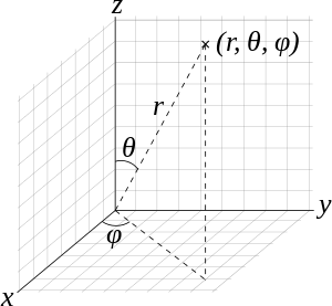
Cylindrical and spherical coordinate systems
There are two common methods for extending the polar coordinate system to three dimensions. In the cylindrical coordinate system, a z-coordinate with the same meaning as in Cartesian coordinates is added to the r and θ polar coordinates giving a triple (ρ, φ, z).[7] Spherical coordinates take this a step further by converting the pair of cylindrical coordinates (r, z) to polar coordinates (ρ, φ) giving a triple (ρ, θ, φ).[8]
Homogeneous coordinate system
A point in the plane may be represented in homogeneous coordinates by a triple (x, y, z) where x/z and y/z are the Cartesian coordinates of the point.[9] This introduces an "extra" coordinate since only two are needed to specify a point on the plane, but this system is useful in that it represents any point on the projective plane without the use of infinity. In general, a homogeneous coordinate system is one where only the ratios of the coordinates are significant and not the actual values.
Other commonly used systems
Some other common coordinate systems are the following:
- Curvilinear coordinates are a generalization of coordinate systems generally; the system is based on the intersection of curves.
- Orthogonal coordinates: coordinate surfaces meet at right angles
- Skew coordinates: coordinate surfaces are not orthogonal
- The log-polar coordinate system represents a point in the plane by the logarithm of the distance from the origin and an angle measured from a reference line intersecting the origin.
- Plücker coordinates are a way of representing lines in 3D Euclidean space using a six-tuple of numbers as homogeneous coordinates.
- Generalized coordinates are used in the Lagrangian treatment of mechanics.
- Canonical coordinates are used in the Hamiltonian treatment of mechanics.
- Barycentric coordinates as used for ternary plots and more generally in the analysis of triangles.
- Trilinear coordinates are used in the context of triangles.
There are ways of describing curves without coordinates, using intrinsic equations that use invariant quantities such as curvature and arc length. These include:
- The Whewell equation relates arc length and the tangential angle.
- The Cesàro equation relates arc length and curvature.
Coordinates of geometric objects
Coordinates systems are often used to specify the position of a point, but they may also be used to specify the position of more complex figures such as lines, planes, circles or spheres. For example, Plücker coordinates are used to determine the position of a line in space.[10] When there is a need, the type of figure being described is used to distinguish the type of coordinate system, for example the term line coordinates is used for any coordinate system that specifies the position of a line.
It may occur that systems of coordinates for two different sets of geometric figures are equivalent in terms of their analysis. An example of this is the systems of homogeneous coordinates for points and lines in the projective plane. The two systems in a case like this are said to be dualistic. Dualistic systems have the property that results from one system can be carried over to the other since these results are only different interpretations of the same analytical result; this is known as the principle of duality.[11]
Transformations
Because there are often many different possible coordinate systems for describing geometrical figures, it is important to understand how they are related. Such relations are described by coordinate transformations which give formulas for the coordinates in one system in terms of the coordinates in another system. For example, in the plane, if Cartesian coordinates (x, y) and polar coordinates (r, θ) have the same origin, and the polar axis is the positive x axis, then the coordinate transformation from polar to Cartesian coordinates is given by x = r cosθ and y = r sinθ.
With every bijection from the space to itself two coordinate transformations can be associated:
- such that the new coordinates of the image of each point are the same as the old coordinates of the original point (the formulas for the mapping are the inverse of those for the coordinate transformation)
- such that the old coordinates of the image of each point are the same as the new coordinates of the original point (the formulas for the mapping are the same as those for the coordinate transformation)
For example, in 1D, if the mapping is a translation of 3 to the right, the first moves the origin from 0 to 3, so that the coordinate of each point becomes 3 less, while the second moves the origin from 0 to −3, so that the coordinate of each point becomes 3 more.
Coordinate lines/curves and planes/surfaces

In two dimensions, if one of the coordinates in a point coordinate system is held constant and the other coordinate is allowed to vary, then the resulting curve is called a coordinate curve. In the Cartesian coordinate system the coordinate curves are, in fact, straight lines, thus coordinate lines. Specifically, they are the lines parallel to one of the coordinate axes. For other coordinate systems the coordinates curves may be general curves. For example, the coordinate curves in polar coordinates obtained by holding r constant are the circles with center at the origin. Coordinates systems for Euclidean space other than the Cartesian coordinate system are called curvilinear coordinate systems.[12] This procedure does not always make sense, for example there are no coordinate curves in a homogeneous coordinate system.
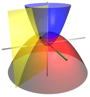
In three-dimensional space, if one coordinate is held constant and the other two are allowed to vary, then the resulting surface is called a coordinate surface. For example, the coordinate surfaces obtained by holding ρ constant in the spherical coordinate system are the spheres with center at the origin. In three-dimensional space the intersection of two coordinate surfaces is a coordinate curve. In the Cartesian coordinate system we may speak of coordinate planes.
Similarly, coordinate hypersurfaces are the n-1-dimensional spaces resulting from fixing a single coordinate of an n-dimensional coordinate system.[13]
Coordinate maps
The concept of a coordinate map, or coordinate chart is central to the theory of manifolds. A coordinate map is essentially a coordinate system for a subset of a given space with the property that each point has exactly one set of coordinates. More precisely, a coordinate map is a homeomorphism from an open subset of a space X to an open subset of Rn.[14] It is often not possible to provide one consistent coordinate system for an entire space. In this case, a collection of coordinate maps are put together to form an atlas covering the space. A space equipped with such an atlas is called a manifold and additional structure can be defined on a manifold if the structure is consistent where the coordinate maps overlap. For example, a differentiable manifold is a manifold where the change of coordinates from one coordinate map to another is always a differentiable function.
Orientation-based coordinates
In geometry and kinematics, coordinate systems are used not only to describe the (linear) position of points, but also to describe the angular position of axes, planes, and rigid bodies.[15] In the latter case, the orientation of a second (typically referred to as "local") coordinate system, fixed to the node, is defined based on the first (typically referred to as "global" or "world" coordinate system). For instance, the orientation of a rigid body can be represented by an orientation matrix, which includes, in its three columns, the Cartesian coordinates of three points. These points are used to define the orientation of the axes of the local system; they are the tips of three unit vectors aligned with those axes.
See also
- Absolute angular momentum
- Alpha-numeric grid
- Analytic geometry
- Astronomical coordinate systems
- Axes conventions in engineering
- Coordinate-free
- Fractional coordinates
- Frame of reference
- Galilean transformation
- Geographic coordinate system
- Nomogram, graphical representations of different coordinate systems
- Rotation of axes
- Translation of axes
Relativistic Coordinate Systems
- Eddington–Finkelstein coordinates
- Gaussian polar coordinates
- Gullstrand–Painlevé coordinates
- Isotropic coordinates
- Kruskal–Szekeres coordinates
- Schwarzschild coordinates
Notes
- ↑ Woods p. 1
- ↑ Weisstein, Eric W. "Coordinate System". MathWorld.
- ↑ Weisstein, Eric W. "Coordinates". MathWorld.
- ↑ Stewart, James B.; Redlin, Lothar; Watson, Saleem (2008). College Algebra (5th ed.). Brooks Cole. pp. 13–19. ISBN 0-495-56521-0.
- ↑ Moon P, Spencer DE (1988). "Rectangular Coordinates (x, y, z)". Field Theory Handbook, Including Coordinate Systems, Differential Equations, and Their Solutions (corrected 2nd, 3rd print ed.). New York: Springer-Verlag. pp. 9–11 (Table 1.01). ISBN 978-0-387-18430-2.
- ↑ Finney, Ross; George Thomas; Franklin Demana; Bert Waits (June 1994). Calculus: Graphical, Numerical, Algebraic (Single Variable Version ed.). Addison-Wesley Publishing Co. ISBN 0-201-55478-X.
- ↑ Margenau, Henry; Murphy, George M. (1956). The Mathematics of Physics and Chemistry. New York City: D. van Nostrand. p. 178. ISBN 9780882754239. LCCN 55010911. OCLC 3017486.
- ↑ Morse PM, Feshbach H (1953). Methods of Theoretical Physics, Part I. New York: McGraw-Hill. p. 658. ISBN 0-07-043316-X. LCCN 52011515.
- ↑ Jones, Alfred Clement (1912). An Introduction to Algebraical Geometry. Clarendon.
- ↑ Hodge, W. V. D.; D. Pedoe (1994) [1947]. Methods of Algebraic Geometry, Volume I (Book II). Cambridge University Press. ISBN 978-0-521-46900-5.
- ↑ Woods p. 2
- ↑ Tang, K. T. (2006). Mathematical Methods for Engineers and Scientists. 2. Springer. p. 13. ISBN 3-540-30268-9.
- ↑ Liseikin, Vladimir D. (2007). A Computational Differential Geometry Approach to Grid Generation. Springer. p. 38. ISBN 3-540-34235-4.
- ↑ Munkres, James R. (2000) Topology. Prentice Hall. ISBN 0-13-181629-2.
- ↑ Hanspeter Schaub; John L. Junkins (2003). "Rigid body kinematics". Analytical Mechanics of Space Systems. American Institute of Aeronautics and Astronautics. p. 71. ISBN 1-56347-563-4.
References
- Voitsekhovskii, M.I.; Ivanov, A.B. (2001), "Coordinates", in Hazewinkel, Michiel, Encyclopedia of Mathematics, Springer, ISBN 978-1-55608-010-4
- Woods, Frederick S. (1922). Higher Geometry. Ginn and Co. pp. 1ff.
- Shigeyuki Morita; Teruko Nagase; Katsumi Nomizu (2001). Geometry of Differential Forms. AMS Bookstore. p. 12. ISBN 0-8218-1045-6.
External links
| Look up coordinate in Wiktionary, the free dictionary. |
| Wikimedia Commons has media related to Coordinate systems. |