Ideal gas
| Thermodynamics | ||||||||||||
|---|---|---|---|---|---|---|---|---|---|---|---|---|
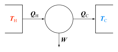 The classical Carnot heat engine | ||||||||||||
|
Branches |
||||||||||||
|
||||||||||||
| Book:Thermodynamics | ||||||||||||


An ideal gas is a theoretical gas composed of many randomly moving point particles that do not interact except when they collide elastically. The ideal gas concept is useful because it obeys the ideal gas law, a simplified equation of state, and is amenable to analysis under statistical mechanics. One mole of an ideal gas has a volume of 22.4 litres at STP as defined by IUPAC.
At normal conditions such as standard temperature and pressure, most real gases behave qualitatively like an ideal gas. Many gases such as nitrogen, oxygen, hydrogen, noble gases, and some heavier gases like carbon dioxide can be treated like ideal gases within reasonable tolerances.[1] Generally, a gas behaves more like an ideal gas at higher temperature and lower pressure,[1] as the potential energy due to intermolecular forces becomes less significant compared with the particles' kinetic energy, and the size of the molecules becomes less significant compared to the empty space between them.
The ideal gas model tends to fail at lower temperatures or higher pressures, when intermolecular forces and molecular size become important. It also fails for most heavy gases, such as many refrigerants,[1] and for gases with strong intermolecular forces, notably water vapor. At high pressures, the volume of a real gas is often considerably greater than that of an ideal gas. At low temperatures, the pressure of a real gas is often considerably less than that of an ideal gas. At some point of low temperature and high pressure, real gases undergo a phase transition, such as to a liquid or a solid. The model of an ideal gas, however, does not describe or allow phase transitions. These must be modeled by more complex equations of state. The deviation from the ideal gas behaviour can be described by a dimensionless quantity, the compressibility factor, Z.
The ideal gas model has been explored in both the Newtonian dynamics (as in "kinetic theory") and in quantum mechanics (as a "gas in a box"). The ideal gas model has also been used to model the behavior of electrons in a metal (in the Drude model and the free electron model), and it is one of the most important models in statistical mechanics.
Types of ideal gas
There are three basic classes of ideal gas:
- the classical or Maxwell–Boltzmann ideal gas,
- the ideal quantum Bose gas, composed of bosons, and
- the ideal quantum Fermi gas, composed of fermions.
The classical ideal gas can be separated into two types: The classical thermodynamic ideal gas and the ideal quantum Boltzmann gas. Both are essentially the same, except that the classical thermodynamic ideal gas is based on classical statistical mechanics, and certain thermodynamic parameters such as the entropy are only specified to within an undetermined additive constant. The ideal quantum Boltzmann gas overcomes this limitation by taking the limit of the quantum Bose gas and quantum Fermi gas in the limit of high temperature to specify these additive constants. The behavior of a quantum Boltzmann gas is the same as that of a classical ideal gas except for the specification of these constants. The results of the quantum Boltzmann gas are used in a number of cases including the Sackur–Tetrode equation for the entropy of an ideal gas and the Saha ionization equation for a weakly ionized plasma.
Classical thermodynamic ideal gas
Macroscopic account
The ideal gas law is an extension of experimentally discovered gas laws. Real fluids at low density and high temperature approximate the behavior of a classical ideal gas. However, at lower temperatures or a higher density, a real fluid deviates strongly from the behavior of an ideal gas, particularly as it condenses from a gas into a liquid or as it deposits from a gas into a solid. This deviation is expressed as a compressibility factor.
The classical thermodynamic properties of an ideal gas can be described by two equations of state:.[2][3]
One of them is the well known ideal gas law

where
- P is the pressure
- V is the volume
- n is the amount of substance of the gas (in moles)
- R is the gas constant (8.314 J·K−1·mol−1)
- T is the absolute temperature.
This equation is derived from Boyle's law: V = k/P (at constant T and n); Charles's law: V = bT (at constant P and n); and Avogadro's law: V = an (at constant T and P); where
- k is a constant used in Boyle's law
- b is a proportionality constant; equal to V/T
- a is a proportionality constant; equal to V/n.
Multiplying the equations representing the three laws:

Gives:
- .

Under ideal conditions,
- ;

that is,
- .

The other equation of state of an ideal gas must express Joule's law, that the internal energy of a fixed mass of ideal gas is a function only of its temperature. For the present purposes it is convenient to postulate an exemplary version of this law by writing:

where
- U is the internal energy
- ĉV is the dimensionless specific heat capacity at constant volume, approximately 3/2 for a monatomic gas, 5/2 for diatomic gas, and 7/2 for more complex molecules.
Microscopic model
In order to switch from macroscopic quantities (left hand side of the following equation) to microscopic ones (right hand side), we use

where
- N is the number of gas particles
- kB is the Boltzmann constant (1.381×10⁻²³ J·K−1).
The probability distribution of particles by velocity or energy is given by the Maxwell speed distribution.
The ideal gas model depends on the following assumptions:
- The molecules of the gas are indistinguishable, small, hard spheres
- All collisions are elastic and all motion is frictionless (no energy loss in motion or collision)
- Newton's laws apply
- The average distance between molecules is much larger than the size of the molecules
- The molecules are constantly moving in random directions with a distribution of speeds
- There are no attractive or repulsive forces between the molecules apart from those that determine their point-like collisions
- The only forces between the gas molecules and the surroundings are those that determine the point-like collisions of the molecules with the walls
- In the simplest case, there are no long-range forces between the molecules of the gas and the surroundings.
The assumption of spherical particles is necessary so that there are no rotational modes allowed, unlike in a diatomic gas. The following three assumptions are very related: molecules are hard, collisions are elastic, and there are no inter-molecular forces. The assumption that the space between particles is much larger than the particles themselves is of paramount importance, and explains why the ideal gas approximation fails at high pressures.
Heat capacity
The heat capacity at constant volume, including an ideal gas is:

where S is the entropy. This is the dimensionless heat capacity at constant volume, which is generally a function of temperature due to intermolecular forces. For moderate temperatures, the constant for a monatomic gas is ĉV = 3/2 while for a diatomic gas it is ĉV = 5/2. It is seen that macroscopic measurements on heat capacity provide information on the microscopic structure of the molecules.
The heat capacity at constant pressure of 1/R mole of ideal gas is:

where H = U + PV is the enthalpy of the gas.
Sometimes, a distinction is made between an ideal gas, where ĉV and ĉP could vary with temperature, and a perfect gas, for which this is not the case.
The ratio of the constant volume and constant pressure heat capacity is

For air, which is a mixture of gases, this ratio is 1.4.
Entropy
Using the results of thermodynamics only, we can go a long way in determining the expression for the entropy of an ideal gas. This is an important step since, according to the theory of thermodynamic potentials, if we can express the entropy as a function of U (U is a thermodynamic potential), volume V and the number of particles N, then we will have a complete statement of the thermodynamic behavior of the ideal gas. We will be able to derive both the ideal gas law and the expression for internal energy from it.
Since the entropy is an exact differential, using the chain rule, the change in entropy when going from a reference state 0 to some other state with entropy S may be written as ΔS where:

where the reference variables may be functions of the number of particles N. Using the definition of the heat capacity at constant volume for the first differential and the appropriate Maxwell relation for the second we have:

Expressing CV in terms of ĉV as developed in the above section, differentiating the ideal gas equation of state, and integrating yields:

which implies that the entropy may be expressed as:

where all constants have been incorporated into the logarithm as f(N) which is some function of the particle number N having the same dimensions as VTĉV in order that the argument of the logarithm be dimensionless. We now impose the constraint that the entropy be extensive. This will mean that when the extensive parameters (V and N) are multiplied by a constant, the entropy will be multiplied by the same constant. Mathematically:

From this we find an equation for the function f(N)

Differentiating this with respect to a, setting a equal to 1, and then solving the differential equation yields f(N):

where Φ may vary for different gases, but will be independent of the thermodynamic state of the gas. It will have the dimensions of VTĉV/N. Substituting into the equation for the entropy:

and using the expression for the internal energy of an ideal gas, the entropy may be written:
![{\displaystyle {\frac {S}{Nk}}=\ln \left[{\frac {V}{N}}\,\left({\frac {U}{{\hat {c}}_{V}kN}}\right)^{{\hat {c}}_{V}}\,{\frac {1}{\Phi }}\right]}](../I/m/65d5055ff166a2ab540fb032ec1d0ace534b5966.svg)
Since this is an expression for entropy in terms of U, V, and N, it is a fundamental equation from which all other properties of the ideal gas may be derived.
This is about as far as we can go using thermodynamics alone. Note that the above equation is flawed — as the temperature approaches zero, the entropy approaches negative infinity, in contradiction to the third law of thermodynamics. In the above "ideal" development, there is a critical point, not at absolute zero, at which the argument of the logarithm becomes unity, and the entropy becomes zero. This is unphysical. The above equation is a good approximation only when the argument of the logarithm is much larger than unity — the concept of an ideal gas breaks down at low values of V/N. Nevertheless, there will be a "best" value of the constant in the sense that the predicted entropy is as close as possible to the actual entropy, given the flawed assumption of ideality. A quantum-mechanical derivation of this constant is developed in the derivation of the Sackur–Tetrode equation which expresses the entropy of a monatomic (ĉV = 3/2) ideal gas. In the Sackur–Tetrode theory the constant depends only upon the mass of the gas particle. The Sackur–Tetrode equation also suffers from a divergent entropy at absolute zero, but is a good approximation for the entropy of a monatomic ideal gas for high enough temperatures.
Thermodynamic potentials
Expressing the entropy as a function of T, V, and N:

The chemical potential of the ideal gas is calculated from the corresponding equation of state (see thermodynamic potential):

where G is the Gibbs free energy and is equal to U + PV − TS so that:

The thermodynamic potentials for an ideal gas can now be written as functions of T, V, and N as:


where, as before,
- .

The most informative way of writing the potentials is in terms of their natural variables, since each of these equations can be used to derive all of the other thermodynamic variables of the system. In terms of their natural variables, the thermodynamic potentials of a single-species ideal gas are:


In statistical mechanics, the relationship between the Helmholtz free energy and the partition function is fundamental, and is used to calculate the thermodynamic properties of matter; see configuration integral for more details.
Speed of sound
The speed of sound in an ideal gas is given by

where
- γ is the adiabatic index (ĉP/ĉV)
- s is the entropy per particle of the gas.
- ρ is the mass density of the gas.
- P is the pressure of the gas.
- R is the universal gas constant
- T is the temperature
- M is the molar mass of the gas.
Table of ideal gas equations
See Table of thermodynamic equations: Ideal gas.
Ideal quantum gases
In the above-mentioned Sackur–Tetrode equation, the best choice of the entropy constant was found to be proportional to the quantum thermal wavelength of a particle, and the point at which the argument of the logarithm becomes zero is roughly equal to the point at which the average distance between particles becomes equal to the thermal wavelength. In fact, quantum theory itself predicts the same thing. Any gas behaves as an ideal gas at high enough temperature and low enough density, but at the point where the Sackur–Tetrode equation begins to break down, the gas will begin to behave as a quantum gas, composed of either bosons or fermions. (See the gas in a box article for a derivation of the ideal quantum gases, including the ideal Boltzmann gas.)
Gases tend to behave as an ideal gas over a wider range of pressures when the temperature reaches the Boyle temperature.
Ideal Boltzmann gas
The ideal Boltzmann gas yields the same results as the classical thermodynamic gas, but makes the following identification for the undetermined constant Φ:

where Λ is the thermal de Broglie wavelength of the gas and g is the degeneracy of states.
Ideal Bose and Fermi gases
An ideal gas of bosons (e.g. a photon gas) will be governed by Bose–Einstein statistics and the distribution of energy will be in the form of a Bose–Einstein distribution. An ideal gas of fermions will be governed by Fermi–Dirac statistics and the distribution of energy will be in the form of a Fermi–Dirac distribution.
See also
- Compressibility factor
- Dynamical billiards – billiard balls as a model of an ideal gas
- Table of thermodynamic equations
- Scale-free ideal gas
References
- 1 2 3 Cengel, Yunus A.; Boles, Michael A. Thermodynamics: An Engineering Approach (4th ed.). p. 89. ISBN 0-07-238332-1.
- ↑ Adkins, C. J. (1983). Equilibrium Thermodynamics (3rd ed.). Cambridge, UK: Cambridge University Press. p. 116–120. ISBN 0-521-25445-0.
- ↑ Tschoegl, N. W. (2000). Fundamentals of Equilibrium and Steady-State Thermodynamics. Amsterdam: Elsevier. p. 88. ISBN 0-444-50426-5.