Yamabe invariant

In mathematics, in the field of differential geometry, the Yamabe invariant (also referred to as the sigma constant) is a real number invariant associated to a smooth manifold that is preserved under diffeomorphisms. It was first written down independently by O. Kobayashi and R. Schoen and takes its name from H. Yamabe.

Definition

Let $M$ be a compact smooth manifold (without boundary) of dimension $n\geq 2$ . The normalized Einstein–Hilbert functional $\mathcal{E}$ assigns to each Riemannian metric $g$ on $M$ a real number as follows:

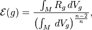
\mathcal{E}(g) = \frac{\int_M R_g \, dV_g}{\left(\int_M \, dV_g\right)^{\frac{n-2}{n}}},

where $R_g$ is the scalar curvature of $g$ and $dV_g$ is the volume density associated to the metric $g$ . The exponent in the denominator is chosen so that the functional is scale-invariant: for every positive real constant $c$ , it satisfies 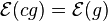$\mathcal{E}(cg) = \mathcal{E}(g)$ . We may think of $\mathcal{E}(g)$ as measuring the average scalar curvature of $g$ over $M$ . It was conjectured by Yamabe that every conformal class of metrics contains a metric of constant scalar curvature (the so-called Yamabe problem); it was proven by Yamabe, Trudinger, Aubin, and Schoen that a minimum value of $\mathcal{E}(g)$ is attained in each conformal class of metrics, and in particular this minimum is achieved by a metric of constant scalar curvature.

We define

Y(g) = \inf_{f} \mathcal{E}(e^{2f} g),

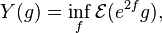
where the infimum is taken over the smooth real-valued functions $f$ on $M$ . This infimum is finite (not $-\infty$ ): Hölder's inequality implies 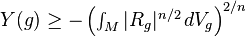$Y(g) \geq -\left(\textstyle\int_M |R_g|^{n/2} \,dV_g\right)^{2/n}$ . The number $Y(g)$ is sometimes called the conformal Yamabe energy of $g$ (and is constant on conformal classes).

A comparison argument due to Aubin shows that for any metric $g$ , $Y(g)$ is bounded above by $\mathcal{E}(g_0)$ , where $g_0$ is the standard metric on the $n$ -sphere $S^n$ . It follows that if we define

\sigma(M) = \sup_{g} Y(g),

where the supremum is taken over all metrics on $M$ , then $\sigma(M) \leq \mathcal{E}(g_0)$ (and is in particular finite). The real number $\sigma(M)$ is called the Yamabe invariant of $M$ .

The Yamabe invariant in two dimensions

In the case that $n=2$ , (so that M is a closed surface) the Einstein–Hilbert functional is given by

\mathcal{E}(g) = \int_M R_g \, dV_g = \int_M 2K_g \, dV_g,

where $K_g$ is the Gauss curvature of g. However, by the Gauss–Bonnet theorem, the integral of the Gauss curvature is given by $2\pi \chi(M)$ , where $\chi(M)$ is the Euler characteristic of M. In particular, this number does not depend on the choice of metric. Therefore, for surfaces, we conclude that

\sigma(M) = 4\pi \chi(M).

For example, the 2-sphere has Yamabe invariant equal to $8\pi$ , and the 2-torus has Yamabe invariant equal to zero.

Examples

In the late 1990s, the Yamabe invariant was computed for large classes of 4-manifolds by Claude LeBrun and his collaborators. In particular, it was shown that most compact complex surfaces have negative, exactly computable Yamabe invariant, and that any Kähler–Einstein metric of negative scalar curvature realizes the Yamabe invariant in dimension 4. It was also shown that the Yamabe invariant of $CP^2$ is realized by the Fubini–Study metric, and so is less than that of the 4-sphere. Most of these arguments involve Seiberg–Witten theory, and so are specific to dimension 4.

An important result due to Petean states that if $M$ is simply connected and has dimension $n \geq 5$ , then $\sigma (M) \geq 0$ . In light of Perelman's solution of the Poincaré conjecture, it follows that a simply connected $n$ -manifold can have negative Yamabe invariant only if $n=4$ . On the other hand, as has already been indicated, simply connected $4$ -manifolds do in fact often have negative Yamabe invariants.

Below is a table of some smooth manifolds of dimension three with known Yamabe invariant. In dimension 3, the number $\mathcal{E}(g_0)$ is equal to $6(2\pi^2)^{2/3}$ and is often denoted $\sigma_1$ .

$M$	$\sigma(M)$	notes
$S^3$	$\sigma_1$	the 3-sphere
$S^2 \times S^1$	$\sigma_1$	the trivial 2-sphere bundle over $S^1$ ^[1]
$S^2 \stackrel{\sim}{\times} S^1$	$\sigma_1$	the unique non-orientable 2-sphere bundle over $S^1$
$\R \mathbb{P}^3$	$\sigma_1/2^{2/3}$	computed by Bray and Neves
$\R \mathbb{P}^2 \times S^1$	$\sigma_1/2^{2/3}$	computed by Bray and Neves
$T^3$	$0$	the 3-torus

By an argument due to Anderson, Perelman's results on the Ricci flow imply that the constant-curvature metric on any hyperbolic 3-manifold realizes the Yamabe invariant. This provides us with infinitely many examples of 3-manifolds for which the invariant is both negative and exactly computable.

Topological significance

The sign of the Yamabe invariant of $M$ holds important topological information. For example, $\sigma(M)$ is positive if and only if $M$ admits a metric of positive scalar curvature.^[2] The significance of this fact is that much is known about the topology of manifolds with metrics of positive scalar curvature.

Notes

↑ See Schoen, pg. 135
↑ Akutagawa, et al., pg. 73

References

M.T. Anderson, "Canonical metrics on 3-manifolds and 4-manifolds", Asian J. Math. 10 127–163 (2006).
K. Akutagawa, M. Ishida, and C. LeBrun, "Perelman's invariant, Ricci flow, and the Yamabe invariants of smooth manifolds", Arch. Math. 88, 71–76 (2007).
H. Bray and A. Neves, "Classification of prime 3-manifolds with Yamabe invariant greater than $\mathbb{RP}^3$ ", Ann. of Math. 159, 407–424 (2004).
M.J. Gursky and C. LeBrun, "Yamabe invariants and $Spin^c$ structures", Geom. Funct. Anal. 8965–977 (1998).
O. Kobayashi, "Scalar curvature of a metric with unit volume", Math. Ann. 279, 253–265, 1987.
C. LeBrun, "Four-manifolds without Einstein metrics", Math. Res. Lett. 3 133–147 (1996).
C. LeBrun, "Kodaira dimension and the Yamabe problem," Comm. Anal. Geom. 7 133–156 (1999).
J. Petean, "The Yamabe invariant of simply connected manifolds", J. Reine Angew. Math. 523 225–231 (2000).
R. Schoen, "Variational theory for the total scalar curvature functional for Riemannian metrics and related topics", Topics in calculus of variations, Lect. Notes Math. 1365, Springer, Berlin, 120–154, 1989.

This article is issued from Wikipedia - version of the 12/21/2014. The text is available under the Creative Commons Attribution/Share Alike but additional terms may apply for the media files.