Yield surface


A yield surface is a five-dimensional surface in the six-dimensional space of stresses. The yield surface is usually convex and the state of stress of inside the yield surface is elastic. When the stress state lies on the surface the material is said to have reached its yield point and the material is said to have become plastic. Further deformation of the material causes the stress state to remain on the yield surface, even though the shape and size of the surface may change as the plastic deformation evolves. This is because stress states that lie outside the yield surface are non-permissible in rate-independent plasticity, though not in some models of viscoplasticity.[1]
The yield surface is usually expressed in terms of (and visualized in) a three-dimensional principal stress space (), a two- or three-dimensional space spanned by stress invariants () or a version of the three-dimensional Haigh–Westergaard stress space. Thus we may write the equation of the yield surface (that is, the yield function) in the forms:


- where are the principal stresses.
- where is the first principal invariant of the Cauchy stress and are the second and third principal invariants of the deviatoric part of the Cauchy stress.
- where are scaled versions of and and is a function of .
- where are scaled versions of and , and is the Lode angle.


Invariants used to describe yield surfaces


The first principal invariant () of the Cauchy stress (), and the second and third principal invariants () of the deviatoric part () of the Cauchy stress are defined as:


![\begin{align}
I_1 & = \text{Tr}(\boldsymbol{\sigma}) = \sigma_1 + \sigma_2 + \sigma_3 \\
J_2 & = \tfrac{1}{2} \boldsymbol{s}:\boldsymbol{s} =
\tfrac{1}{6}\left[(\sigma_1-\sigma_2)^2+(\sigma_2-\sigma_3)^2+(\sigma_3-\sigma_1)^2\right] \\
J_3 & = \det(\boldsymbol{s}) = \tfrac{1}{3} (\boldsymbol{s}\cdot\boldsymbol{s}):\boldsymbol{s}
= s_1 s_2 s_3
\end{align}](../I/m/2367aae106ad4915a3c05e829c4d06e62ee17c18.svg)
where () are the principal values of , () are the principal values of , and


where is the identity matrix.

A related set of quantities, (), are usually used to describe yield surfaces for cohesive frictional materials such as rocks, soils, and ceramics. These are defined as


where is the equivalent stress. However, the possibility of negative values of and the resulting imaginary makes the use of these quantities problematic in practice.

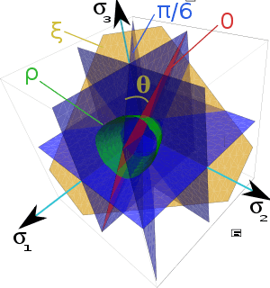
Another related set of widely used invariants is () which describe a cylindrical coordinate system (the Haigh–Westergaard coordinates). These are defined as:


The plane is also called the Rendulic plane. The angle is called the Lode angle[2] and the relation between and was first given by Nayak and Zienkiewicz in 1972 [3]

The principal stresses and the Haigh–Westergaard coordinates are related by

A different definition of the Lode angle can also be found in the literature:[4]

in which case the ordered principal stresses (where ) are related by[5]


Examples of yield surfaces
There are several different yield surfaces known in engineering, and those most popular are listed below.
Tresca yield surface
The Tresca yield criterion is taken to be the work of Henri Tresca.[6] It is also known as the maximum shear stress theory (MSST) and the Tresca–[7] (TG) criterion. In terms of the principal stresses the Tresca criterion is expressed as

Where is the yield strength in shear, and is the tensile yield strength.


Figure 1 shows the Tresca–Guest yield surface in the three-dimensional space of principal stresses. It is a prism of six sides and having infinite length. This means that the material remains elastic when all three principal stresses are roughly equivalent (a hydrostatic pressure), no matter how much it is compressed or stretched. However, when one of the principal stresses becomes smaller (or larger) than the others the material is subject to shearing. In such situations, if the shear stress reaches the yield limit then the material enters the plastic domain. Figure 2 shows the Tresca–Guest yield surface in two-dimensional stress space, it is a cross section of the prism along the plane.

 Figure 1: View of Tresca–Guest yield surface in 3D space of principal stresses
 Figure 2: Tresca–Guest yield surface in 2D space ()
von Mises yield surface
The von Mises yield criterion is expressed in the principal stresses as

where is the yield strength in uniaxial tension.
Figure 3 shows the von Mises yield surface in the three-dimensional space of principal stresses. It is a circular cylinder of infinite length with its axis inclined at equal angles to the three principal stresses. Figure 4 shows the von Mises yield surface in two-dimensional space compared with Tresca–Guest criterion. A cross section of the von Mises cylinder on the plane of produces the elliptical shape of the yield surface.
 Figure 3: View of Huber–Mises–Hencky yield surface in 3D space of principal stresses
 Figure 4: Comparison of Tresca–Guest and Huber–Mises–Hencky criteria in 2D space ()
Burzyński-Yagn criterion

represents the general equation of a second order surface of revolution about the hydrostatic axis. Some special case are:[10]
- cylinder (Maxwell (1865), Huber (1904), von Mises (1913), Hencky (1924)),
- cone (Drucker-Prager (1952), Mirolyubov (1953)),
- paraboloid (Burzyński (1928), Balandin (1937), Torre (1947)),
- ellipsoid centered of symmetry plane , (Beltrami (1885)),
- ellipsoid centered of symmetry plane with (Schleicher (1926)),
- hyperboloid of two sheets (Burzynski (1928), Yagn (1931)),
- hyperboloid of one sheet centered of symmetry plane , , (Kuhn (1980))
- hyperboloid of one sheet , (Filonenko-Boroditsch (1960), Gol’denblat-Kopnov (1968), Filin (1975)).

![\gamma_1 = \gamma_2 \in ]0,1[](../I/m/66ab6f7a14a52c2042d17030aa16705df21f1541.svg)
![\gamma_1 \in ]0,1[, \gamma_2 = 0](../I/m/ab67fc470c16fd7d16b50462f9c9d7af9b70f566.svg)

![\gamma_1 = - \gamma_2 \in ]0,1[](../I/m/19f234ad4d2cddbc2eb4b2b5c0dfcb2a128c275b.svg)

![\gamma_1 \in ]0,1[, \gamma_2<0](../I/m/cc95c96fba08cb97251ef453346323702300f9ab.svg)
![\gamma_1 \in ]0,1[, \gamma_2 \in ]0,\gamma_1[](../I/m/7bdf157e5b65de316f3462bcb5e2de9d10cda1cb.svg)


The relations compression-tension and torsion-tension compute to

The Poisson's ratios at tension and compression are obtained using


For ductile materials the restriction
![\nu_+^\mathrm{in}\in \bigg[\,0.48,\,\frac{1}{2}\,\bigg]](../I/m/4b7c270b90d3c766fd6ecd9b7204e1622d9f7722.svg)
is important. The application of rotationally symmetric models for brittle failure with
![\nu_+^\mathrm{in}\in ]-1,~\nu_+^\mathrm{el}\,]](../I/m/690096f2ce81fb70324e3cebefabb993721ed772.svg)
has not been studied sufficiently.[11]
The Burzyński-Yagn criterion is well suited for academic purposes. For practical applications, the third invariant of the deviator should be introduced, e.g.

Mohr–Coulomb yield surface
The Mohr–Coulomb yield (failure) criterion is similar to the Tresca criterion, with additional provisions for materials with different tensile and compressive yield strengths. This model is often used to model concrete, soil or granular materials. The Mohr–Coulomb yield criterion may be expressed as:

where

and the parameters and are the yield (failure) stresses of the material in uniaxial compression and tension, respectively. The formula reduces to the Tresca criterion if .


Figure 5 shows Mohr–Coulomb yield surface in the three-dimensional space of principal stresses. It is a conical prism and determines the inclination angle of conical surface. Figure 6 shows Mohr–Coulomb yield surface in two-dimensional stress space. It is a cross section of this conical prism on the plane of .

 Figure 5: View of Mohr–Coulomb yield surface in 3D space of principal stresses
 Figure 6: Mohr–Coulomb yield surface in 2D space ()
Drucker–Prager yield surface
The Drucker–Prager yield criterion is similar to the von Mises yield criterion, with provisions for handling materials with differing tensile and compressive yield strengths. This criterion is most often used for concrete where both normal and shear stresses can determine failure. The Drucker–Prager yield criterion may be expressed as

where

and , are the uniaxial yield stresses in compression and tension respectively. The formula reduces to the von Mises equation if .
Figure 7 shows Drucker–Prager yield surface in the three-dimensional space of principal stresses. It is a regular cone. Figure 8 shows Drucker–Prager yield surface in two-dimensional space. The elliptical elastic domain is a cross section of the cone on the plane of ; it can be chosen to intersect the Mohr–Coulomb yield surface in different number of vertices. One choice is to intersect the Mohr–Coulomb yield surface at three vertices on either side of the line, but usually selected by convention to be those in the compression regime.[12] Another choice is to intersect the Mohr–Coulomb yield surface at four vertices on both axes (uniaxial fit) or at two vertices on the diagonal (biaxial fit).[13] The Drucker-Prager yield criterion is also commonly expressed in terms of the material cohesion and friction angle.


 Figure 7: View of Drucker–Prager yield surface in 3D space of principal stresses
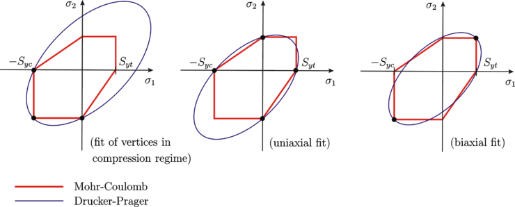 Figure 8: View of Drucker–Prager yield surface in 2D space of principal stresses
Bresler–Pister yield surface
The Bresler–Pister yield criterion is an extension of the Drucker Prager yield criterion that uses three parameters, and has additional terms for materials that yield under hydrostatic compression. In terms of the principal stresses, this yield criterion may be expressed as
![S_{yc} = \tfrac{1}{\sqrt{2}}\left[(\sigma_1-\sigma_2)^2+(\sigma_2-\sigma_3)^2+(\sigma_3-\sigma_1)^2\right]^{1/2} - c_0 - c_1~(\sigma_1+\sigma_2+\sigma_3) - c_2~(\sigma_1+\sigma_2+\sigma_3)^2](../I/m/168ce31fef86a9a05a75721a81e088c69edcf24f.svg)
where are material constants. The additional parameter gives the yield surface an ellipsoidal cross section when viewed from a direction perpendicular to its axis. If is the yield stress in uniaxial compression, is the yield stress in uniaxial tension, and is the yield stress in biaxial compression, the parameters can be expressed as


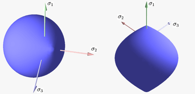 Figure 9: View of Bresler–Pister yield surface in 3D space of principal stresses
 Figure 10: Bresler–Pister yield surface in 2D space ()
Willam–Warnke yield surface
The Willam–Warnke yield criterion is a three-parameter smoothed version of the Mohr–Coulomb yield criterion that has similarities in form to the Drucker–Prager and Bresler–Pister yield criteria.
The yield criterion has the functional form

However, it is more commonly expressed in Haigh–Westergaard coordinates as

The cross-section of the surface when viewed along its axis is a smoothed triangle (unlike Mohr–Coulumb). The Willam–Warnke yield surface is convex and has unique and well defined first and second derivatives on every point of its surface. Therefore, the Willam–Warnke model is computationally robust and has been used for a variety of cohesive-frictional materials.
 Figure 11: View of Willam–Warnke yield surface in 3D space of principal stresses
 Figure 12: Willam–Warnke yield surface in the -plane

Bigoni–Piccolroaz yield surface
The Bigoni–Piccolroaz yield criterion [14][15] is a seven-parameter surface defined by

where is the "meridian" function

![F(p) =
\left\{
\begin{array}{ll}
-M p_c \sqrt{(\phi - \phi^m)[2(1 - \alpha)\phi + \alpha]}, & \phi \in [0,1], \\
+\infty, & \phi \notin [0,1],
\end{array}
\right.](../I/m/9948aa54df1e39ab115e425b19f088dff39beadc.svg)

describing the pressure-sensitivity and is the "deviatoric" function

![g(\theta) = \frac{1}{\cos[\beta \frac{\pi}{6} - \frac{1}{3} \cos^{-1}(\gamma \cos 3\theta)]},](../I/m/dba97f3c7548243d55f4c6736d862e34b31b04cb.svg)
describing the Lode-dependence of yielding. The seven, non-negative material parameters:

define the shape of the meridian and deviatoric sections.
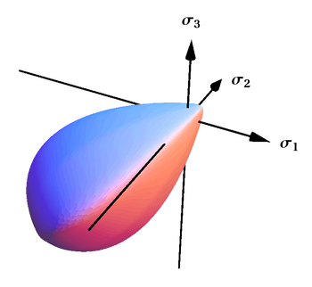
This criterion represents a smooth and convex surface, which is closed both in hydrostatic tension and compression and has a drop-like shape, particularly suited to describe frictional and granular materials. This criterion has also been generalized to the case of surfaces with corners.[16]

Cosine Ansatz Model (Altenbach-Bolchoun-Kolupaev)
For the formulation of the strength hypotheses the stress angle

can be used.
The following model of isotropic material behavior

contains a number of other well-known less general models, provided suitable parameter values are chosen.
Parameters and describe the geometry of the surface in the -plane. They are subject to the constraints


which follow from the convexity condition. A more precise formulation of the third constraints is proposed in.[17]
Parameters and describe the position of the intersection points of the yield surface with hydrostatic axis (space diagonal in the principal stress space). These intersections points are called hydrostatic nodes. In the case of materials which do not fail at hydrostatic pressure (steel, brass, etc.) one gets . Otherwise for materials which fail at hydrostatic pressure (hard foams, ceramics, sintered materials, etc.) it follows .


The integer powers and , describe the curvature of the meridian. The meridian with is a straight line and with - a parabola.


See also
- Yield (engineering)
- Plasticity (physics)
- Stress
- Henri Tresca
- von Mises stress
- Mohr–Coulomb theory
- Strain
- Strain tensor
- Stress–energy tensor
- Stress concentration
- 3-D elasticity
References
- ↑ Simo, J. C. and Hughes, T,. J. R., (1998), Computational Inelasticity, Spinger.
- ↑ Lode, W. (1926). Versuche über den Einfuss der mittleren Hauptspannung auf das Fliessen der Metalle Eisen Kupfer und Nickel. Zeitung Phys., vol. 36, pp. 913–939.
- ↑ Nayak, G. C. and Zienkiewicz, O.C. (1972). Convenient forms of stress invariants for plasticity. Proceedings of the ASCE Journal of the Structural Division, vol. 98, no. ST4, pp. 949–954.
- ↑ Chakrabarty, J., 2006, Theory of Plasticity: Third edition, Elsevier, Amsterdam.
- ↑ Brannon, R.M., 2009, KAYENTA: Theory and User's Guide, Sandia National Laboratories, Albuquerque, New Mexico.
- ↑ Tresca, H. (1864). Mémoire sur l'écoulement des corps solides soumis à de fortes pressions. C.R. Acad. Sci. Paris, vol. 59, p. 754.
- ↑ Guest
- ↑ Burzyński, W. (1929). Über die Anstrengungshypothesen. Schweizerische Bauzeitung, 94 (21), pp. 259-262.
- ↑ Yagn, Yu. I. (1931). New methods of strength prediction (in Russ.: Novye metody pascheta na prochnost'). Vestnik inzhenerov i tekhnikov, 6, pp. 237-244.
- ↑ Altenbach, H., Kolupaev, V.A. (2014) Classical and Non-Classical Failure Criteria, in Altenbach, H., Sadowski, Th., eds., Failure and Damage Analysis of Advanced Materials, in press, Springer, Heidelberg (2014), pp. 1-66
- ↑ Beljaev, N. M. (1979). Strength of Materials. Mir Publ., Moscow
- ↑ Khan and Huang. (1995), Continuum Theory of Plasticity. J.Wiley.
- ↑ Neto, Periç, Owen. (2008), The mathematical Theory of Plasticity. J.Wiley.
- ↑ Bigoni, D. Nonlinear Solid Mechanics: Bifurcation Theory and Material Instability. Cambridge University Press, 2012 . ISBN 9781107025417.
- ↑ Bigoni, D. and Piccolroaz, A., (2004), Yield criteria for quasibrittle and frictional materials, International Journal of Solids and Structures 41, 2855-2878.
- ↑ Piccolroaz, A. and Bigoni, D. (2009), Yield criteria for quasibrittle and frictional materials: a generalization to surfaces with corners, International Journal of Solids and Structures 46, 3587-3596.
- ↑ Altenbach, H., Bolchoun, A., Kolupaev, V.A. (2013). Phenomenological Yield and Failure Criteria, in Altenbach, H., Öchsner, A., eds., Plasticity of Pressure-Sensitive Materials, Serie ASM, Springer, Heidelberg, pp. 49-152.