Chebyshev filter
| Linear analog electronic filters |
|---|
|
|
Simple filters |
Chebyshev filters are analog or digital filters having a steeper roll-off and more passband ripple (type I) or stopband ripple (type II) than Butterworth filters. Chebyshev filters have the property that they minimize the error between the idealized and the actual filter characteristic over the range of the filter, but with ripples in the passband. This type of filter is named after Pafnuty Chebyshev because its mathematical characteristics are derived from Chebyshev polynomials.
Because of the passband ripple inherent in Chebyshev filters, the ones that have a smoother response in the passband but a more irregular response in the stopband are preferred for some applications.
Type I Chebyshev filters
.svg.png)

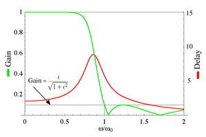
Type I Chebyshev filters are the most common types of Chebyshev filters. The gain (or amplitude) response, , as a function of angular frequency of the nth-order low-pass filter is equal to the absolute value of the transfer function evaluated at :


where is the ripple factor, is the cutoff frequency and is a Chebyshev polynomial of the th order.


The passband exhibits equiripple behavior, with the ripple determined by the ripple factor . In the passband, the Chebyshev polynomial alternates between -1 and 1 so the filter gain alternate between maxima at G = 1 and minima at .

The ripple factor ε is thus related to the passband ripple δ in decibels by:

At the cutoff frequency the gain again has the value but continues to drop into the stopband as the frequency increases. This behavior is shown in the diagram on the right. The common practice of defining the cutoff frequency at −3 dB is usually not applied to Chebyshev filters; instead the cutoff is taken as the point at which the gain falls to the value of the ripple for the final time.

The 3 dB frequency ωH is related to ω0 by:

The order of a Chebyshev filter is equal to the number of reactive components (for example, inductors) needed to realize the filter using analog electronics.
An even steeper roll-off can be obtained if ripple is allowed in the stopband, by allowing zeroes on the -axis in the complex plane. However, this results in less suppression in the stopband. The result is called an elliptic filter, also known as Cauer filter.

Poles and zeroes
.svg.png)

For simplicity, it is assumed that the cutoff frequency is equal to unity. The poles of the gain function of the Chebyshev filter are the zeroes of the denominator of the gain function. Using the complex frequency s, these occur when:


Defining and using the trigonometric definition of the Chebyshev polynomials yields:


Solving for


where the multiple values of the arc cosine function are made explicit using the integer index m. The poles of the Chebyshev gain function are then:


Using the properties of the trigonometric and hyperbolic functions, this may be written in explicitly complex form:


where m = 1, 2,..., n and

This may be viewed as an equation parametric in and it demonstrates that the poles lie on an ellipse in s-space centered at s = 0 with a real semi-axis of length and an imaginary semi-axis of length of


The transfer function
The above expression yields the poles of the gain G. For each complex pole, there is another which is the complex conjugate, and for each conjugate pair there are two more that are the negatives of the pair. The transfer function must be stable, so that its poles are those of the gain that have negative real parts and therefore lie in the left half plane of complex frequency space. The transfer function is then given by

where are only those poles of the gain with a negative sign in front of the real term in the above equation for the poles.

The group delay

The group delay is defined as the derivative of the phase with respect to angular frequency and is a measure of the distortion in the signal introduced by phase differences for different frequencies.

The gain and the group delay for a fifth-order type I Chebyshev filter with ε=0.5 are plotted in the graph on the left. It can be seen that there are ripples in the gain and the group delay in the passband but not in the stopband.
Type II Chebyshev filters


Also known as inverse Chebyshev filters, the Type II Chebyshev filter type is less common because it does not roll off as fast as Type I, and requires more components. It has no ripple in the passband, but does have equiripple in the stopband. The gain is:

In the stopband, the Chebyshev polynomial oscillates between -1 and 1 so that the gain will oscillate between zero and

and the smallest frequency at which this maximum is attained is the cutoff frequency . The parameter ε is thus related to the stopband attenuation γ in decibels by:


For a stopband attenuation of 5 dB, ε = 0.6801; for an attenuation of 10 dB, ε = 0.3333. The frequency f0 = ω0/2π is the cutoff frequency. The 3 dB frequency fH is related to f0 by:

Poles and zeroes
.svg.png)
Assuming that the cutoff frequency is equal to unity, the poles of the gain of the Chebyshev filter are the zeroes of the denominator of the gain:

The poles of gain of the type II Chebyshev filter are the inverse of the poles of the type I filter:


where m = 1, 2, ..., n . The zeroes of the type II Chebyshev filter are the zeroes of the numerator of the gain:


The zeroes of the type II Chebyshev filter are therefore the inverse of the zeroes of the Chebyshev polynomial.

for m = 1, 2, ..., n.
The transfer function
The transfer function is given by the poles in the left half plane of the gain function, and has the same zeroes but these zeroes are single rather than double zeroes.
The group delay
The gain and the group delay for a fifth-order type II Chebyshev filter with ε=0.1 are plotted in the graph on the left. It can be seen that there are ripples in the gain in the stopband but not in the pass band.
Implementation
Cauer topology
A passive LC Chebyshev low-pass filter may be realized using a Cauer topology. The inductor or capacitor values of a nth-order Chebyshev prototype filter may be calculated from the following equations:[1]


G1, Gk are the capacitor or inductor element values. fH, the 3 dB frequency is calculated with:

The coefficients A, γ, β, Ak, and Bk may be calculated from the following equations:

![\beta =\ln \left[\coth \left({\frac {R_{{db}}}{17.37}}\right)\right]](../I/m/a5aa7efa6e099a85b5f2f7c315338a108eb73768.svg)


where RdB is the passband ripple in decibels.

The calculated Gk values may then be converted into shunt capacitors and series inductors as shown on the right, or they may be converted into series capacitors and shunt inductors. For example,
- C1 shunt = G1, L2 series = G2, ...
or
- L1 shunt = G1, C1 series = G2, ...
Note that when G1 is a shunt capacitor or series inductor, G0 corresponds to the input resistance or conductance, respectively. The same relationship holds for Gn+1 and Gn. The resulting circuit is a normalized low-pass filter. Using frequency transformations and impedance scaling, the normalized low-pass filter may be transformed into high-pass, band-pass, and band-stop filters of any desired cutoff frequency or bandwidth.
Digital
As with most analog filters, the Chebyshev may be converted to a digital (discrete-time) recursive form via the bilinear transform. However, as digital filters have a finite bandwidth, the response shape of the transformed Chebyshev is warped. Alternatively, the Matched Z-transform method may be used, which does not warp the response.
Comparison with other linear filters
The following illustration shows the Chebyshev filters next to other common filter types obtained with the same number of coefficients (fifth order):

Chebyshev filters are sharper than the Butterworth filter; they are not as sharp as the elliptic one, but they show fewer ripples over the bandwidth.
See also
Notes
- ↑ Matthaei et. al 1980, p.99
References
- Daniels, Richard W. (1974). Approximation Methods for Electronic Filter Design. New York: McGraw-Hill. ISBN 0-07-015308-6.
- Williams, Arthur B.; Taylors, Fred J. (1988). Electronic Filter Design Handbook. New York: McGraw-Hill. ISBN 0-07-070434-1.
- Matthaei, George L.; Young, Leo; Jones, E. M. T. (1980). Microwave Filters, Impedance-Matching Networks, and Coupling Structures. Norwood, MA: Artech House. ISBN 0-89-006099-1.