Student's t-test

A t-test is any statistical hypothesis test in which the test statistic follows a Student's t-distribution under the null hypothesis. It can be used to determine if two sets of data are significantly different from each other.

A t-test is most commonly applied when the test statistic would follow a normal distribution if the value of a scaling term in the test statistic were known. When the scaling term is unknown and is replaced by an estimate based on the data, the test statistics (under certain conditions) follow a Student's t distribution.

History

William Sealy Gosset, who developed the "t-statistic" and published it under the pseudonym of "Student".

The t-statistic was introduced in 1908 by William Sealy Gosset, a chemist working for the Guinness brewery in Dublin, Ireland ("Student" was his pen name).^[1]^[2]^[3]^[4]

Gosset had been hired due to Claude Guinness's policy of recruiting the best graduates from Oxford and Cambridge to apply biochemistry and statistics to Guinness's industrial processes.^[2] Gosset devised the t-test as an economical way to monitor the quality of stout. The Student's t-test work was submitted to and accepted in the journal Biometrika and published in 1908.^[5] Company policy at Guinness forbade its chemists from publishing their findings, so Gosset published his statistical work under the pseudonym "Student" (see Student's t-distribution for a detailed history of this pseudonym, which is not to be confused with the literal term, "student").

Guinness had a policy of allowing technical staff leave for study (so-called "study leave"), which Gosset used during the first two terms of the 1906–1907 academic year in Professor Karl Pearson's Biometric Laboratory at University College London.^[6] Gosset's identity was then known to fellow statisticians and to editor-in-chief Karl Pearson.^[7]

It is not clear how much of the work Gosset performed while he was at Guinness and how much was done when he was on study leave at University College London.

Uses

Among the most frequently used t-tests are:

A one-sample location test of whether the mean of a population has a value specified in a null hypothesis.
A two-sample location test of the null hypothesis such that the means of two populations are equal. All such tests are usually called Student's t-tests, though strictly speaking that name should only be used if the variances of the two populations are also assumed to be equal; the form of the test used when this assumption is dropped is sometimes called Welch's t-test. These tests are often referred to as "unpaired" or "independent samples" t-tests, as they are typically applied when the statistical units underlying the two samples being compared are non-overlapping.^[8]
A test of the null hypothesis that the difference between two responses measured on the same statistical unit has a mean value of zero. For example, suppose we measure the size of a cancer patient's tumor before and after a treatment. If the treatment is effective, we expect the tumor size for many of the patients to be smaller following the treatment. This is often referred to as the "paired" or "repeated measures" t-test:^[8]^[9] see paired difference test.
A test of whether the slope of a regression line differs significantly from 0.

Assumptions

Most t-test statistics have the form $t = Z / s$ , where $Z$ and $s$ are functions of the data. Typically, $Z$ is designed to be sensitive to the alternative hypothesis (i.e., its magnitude tends to be larger when the alternative hypothesis is true), whereas s is a scaling parameter that allows the distribution of $t$ to be determined.

As an example, in the one-sample t-test $t={\sqrt {p}}{\frac {Z}{s}}={\sqrt {p}}{\frac {({\bar {X}}-\mu )/(\sigma /{\sqrt {n}})}{s}}$ , where ${\bar {X}}$ is the sample mean from a sample $X 1, X 2, \dots, X n$ , of size $n$ , $s$ is the ratio of sample standard deviation over population standard deviation, $σ$ is the population standard deviation of the data, and $μ$ is the population mean.

The assumptions underlying a t-test are that

$X$ follows a normal distribution with mean $μ$ and variance $σ 2$
$s 2$ follows a $χ 2$ distribution with $p$ degrees of freedom under the null hypothesis, where $p$ is a positive constant
$Z$ and $s$ are independent.

In a specific type of t-test, these conditions are consequences of the population being studied, and of the way in which the data are sampled. For example, in the t-test comparing the means of two independent samples, the following assumptions should be met:

Each of the two populations being compared should follow a normal distribution. This can be tested using a normality test, such as the Shapiro–Wilk or Kolmogorov–Smirnov test, or it can be assessed graphically using a normal quantile plot.
If using Student's original definition of the t-test, the two populations being compared should have the same variance (testable using F-test, Levene's test, Bartlett's test, or the Brown–Forsythe test; or assessable graphically using a Q–Q plot). If the sample sizes in the two groups being compared are equal, Student's original t-test is highly robust to the presence of unequal variances.^[10] Welch's t-test is insensitive to equality of the variances regardless of whether the sample sizes are similar.
The data used to carry out the test should be sampled independently from the two populations being compared. This is in general not testable from the data, but if the data are known to be dependently sampled (i.e., if they were sampled in clusters), then the classical t-tests discussed here may give misleading results.

Most two-sample t-tests are robust to all but large deviations from the assumptions.^[11]

Unpaired and paired two-sample t-tests

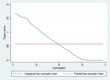
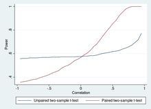
Type I error of unpaired and paired two-sample t-tests as a function of the correlation. The simulated random numbers originate from a bivariate normal distribution with a variance of 1. The significance level is 5% and the number of cases is 60.

Power of unpaired and paired two-sample t-tests as a function of the correlation. The simulated random numbers originate from a bivariate normal distribution with a variance of 1 and a deviation of the expected value of 0.4. The significance level is 5% and the number of cases is 60.

Two-sample t-tests for a difference in mean involve independent samples or unpaired samples. Paired t-tests are a form of blocking, and have greater power than unpaired tests when the paired units are similar with respect to "noise factors" that are independent of membership in the two groups being compared.^[12] In a different context, paired t-tests can be used to reduce the effects of confounding factors in an observational study.

Independent (unpaired) samples

The independent samples t-test is used when two separate sets of independent and identically distributed samples are obtained, one from each of the two populations being compared. For example, suppose we are evaluating the effect of a medical treatment, and we enroll 100 subjects into our study, then randomly assign 50 subjects to the treatment group and 50 subjects to the control group. In this case, we have two independent samples and would use the unpaired form of the t-test. The randomization is not essential here – if we contacted 100 people by phone and obtained each person's age and gender, and then used a two-sample t-test to see whether the mean ages differ by gender, this would also be an independent samples t-test, even though the data is observational.

Paired samples

Main article: Paired difference test

Paired samples t-tests typically consist of a sample of matched pairs of similar units, or one group of units that has been tested twice (a "repeated measures" t-test).

A typical example of the repeated measures t-test would be where subjects are tested prior to a treatment, say for high blood pressure, and the same subjects are tested again after treatment with a blood-pressure lowering medication. By comparing the same patient's numbers before and after treatment, we are effectively using each patient as their own control. That way the correct rejection of the null hypothesis (here: of no difference made by the treatment) can become much more likely, with statistical power increasing simply because the random between-patient variation has now been eliminated. Note however that an increase of statistical power comes at a price: more tests are required, each subject having to be tested twice. Because half of the sample now depends on the other half, the paired version of Student's t-test has only "n/2–1" degrees of freedom (with n being the total number of observations). Pairs become individual test units, and the sample has to be doubled to achieve the same number of degrees of freedom.

A paired samples t-test based on a "matched-pairs sample" results from an unpaired sample that is subsequently used to form a paired sample, by using additional variables that were measured along with the variable of interest.^[13] The matching is carried out by identifying pairs of values consisting of one observation from each of the two samples, where the pair is similar in terms of other measured variables. This approach is sometimes used in observational studies to reduce or eliminate the effects of confounding factors.

Paired samples t-tests are often referred to as "dependent samples t-tests".

Calculations

Explicit expressions that can be used to carry out various t-tests are given below. In each case, the formula for a test statistic that either exactly follows or closely approximates a t-distribution under the null hypothesis is given. Also, the appropriate degrees of freedom are given in each case. Each of these statistics can be used to carry out either a one-tailed or two-tailed test.

Once the t value and degrees of freedom are determined, a p-value can be found using a table of values from Student's t-distribution. If the calculated p-value is below the threshold chosen for statistical significance (usually the 0.10, the 0.05, or 0.01 level), then the null hypothesis is rejected in favor of the alternative hypothesis.

One-sample t-test

In testing the null hypothesis that the population mean is equal to a specified value μ₀, one uses the statistic

t = \frac{\overline{x} - \mu_0}{s/\sqrt{n}}

where ${\overline {x}}$ is the sample mean, s is the sample standard deviation of the sample and n is the sample size. The degrees of freedom used in this test are n − 1. Although the parent population does not need to be normally distributed, the distribution of the population of sample means, $\overline {x}$ , is assumed to be normal. By the central limit theorem, if the sampling of the parent population is independent then the sample means will be approximately normal.^[14] (The degree of approximation will depend on how close the parent population is to a normal distribution and the sample size, n.)

Slope of a regression line

Suppose one is fitting the model

Y=\alpha +\beta x+\varepsilon ,

where x is known, α and β are unknown, and ε is a normally distributed random variable with mean 0 and unknown variance σ², and Y is the outcome of interest. We want to test the null hypothesis that the slope β is equal to some specified value β₀ (often taken to be 0, in which case the null hypothesis is that x and y are independent).

Let

\begin{align} \widehat\alpha, \widehat\beta & = \text{least-squares estimators}, \\ SE_{\widehat\alpha}, SE_{\widehat\beta} & = \text{the standard errors of least-squares estimators}. \end{align}

Then

t_\text{score} = \frac{\widehat\beta - \beta_0}{ SE_{\widehat\beta} }\sim\mathcal{T}_{n-2}

has a t-distribution with n − 2 degrees of freedom if the null hypothesis is true. The standard error of the slope coefficient:

SE_{{\widehat \beta }}={\frac {{\sqrt {{\frac {1}{n-2}}\sum _{{i=1}}^{n}(y_{i}-\widehat y_{i})^{2}}}}{{\sqrt {\sum _{{i=1}}^{n}(x_{i}-\overline {x})^{2}}}}}

can be written in terms of the residuals. Let

{\begin{aligned}\widehat \varepsilon _{i}&=y_{i}-\widehat y_{i}=y_{i}-(\widehat \alpha +\widehat \beta x_{i})={\text{residuals}}={\text{estimated errors}},\\{\text{SSR}}&=\sum _{{i=1}}^{n}\widehat \varepsilon _{i}^{{\;2}}={\text{sum of squares of residuals}}.\end{aligned}}

Then $t_\text{score}$ is given by:

t_\text{score} = \frac{(\widehat\beta - \beta_0)\sqrt{n-2}}{ \sqrt{\text{SSR}/\sum_{i=1}^n \left(x_i - \overline{x}\right)^2} }.

Independent two-sample t-test

Equal sample sizes, equal variance

Given two groups (1, 2), this test is only applicable when:

the two sample sizes (that is, the number, n, of participants of each group) are equal;
it can be assumed that the two distributions have the same variance;

Violations of these assumptions are discussed below.

The t statistic to test whether the means are different can be calculated as follows:

t={\frac {{\bar {X}}_{1}-{\bar {X}}_{2}}{s_{p}{\sqrt {2/n}}}}

where

\ s_{p}={\sqrt {\frac {s_{X_{1}}^{2}+s_{X_{2}}^{2}}{2}}}

Here $s_{p}$ is the pooled standard deviation for n=n₁=n₂ and $s_{X_1}^2$ and $s_{X_2}^2$ are the unbiased estimators of the variances of the two samples. The denominator of t is the standard error of the difference between two means.

For significance testing, the degrees of freedom for this test is 2n − 2 where n is the number of participants in each group.

Equal or unequal sample sizes, equal variance

This test is used only when it can be assumed that the two distributions have the same variance. (When this assumption is violated, see below.) Note that the previous formulae are a special case valid when both samples have equal sizes: n = n₁ = n₂. The t statistic to test whether the means are different can be calculated as follows:

t={\frac {{\bar {X}}_{1}-{\bar {X}}_{2}}{s_{p}\cdot {\sqrt {{\frac {1}{n_{1}}}+{\frac {1}{n_{2}}}}}}}

where

s_{p}={\sqrt {\frac {(n_{1}-1)s_{X_{1}}^{2}+(n_{2}-1)s_{X_{2}}^{2}}{n_{1}+n_{2}-2}}}.

is an estimator of the pooled standard deviation of the two samples: it is defined in this way so that its square is an unbiased estimator of the common variance whether or not the population means are the same. In these formulae, $n i - 1$ is the number of degrees of freedom for each group, and the total sample size minus two (that is, $n 1 + n 2 - 2$ ) is the total number of degrees of freedom, which is used in significance testing.

Equal or unequal sample sizes, unequal variances

Main article: Welch's t-test

This test, also known as Welch's t-test, is used only when the two population variances are not assumed to be equal (the two sample sizes may or may not be equal) and hence must be estimated separately. The t statistic to test whether the population means are different is calculated as:

t={{\overline {X}}_{1}-{\overline {X}}_{2} \over s_{\overline {\Delta }}}

where

s_{\overline {\Delta }}={\sqrt {{s_{1}^{2} \over n_{1}}+{s_{2}^{2} \over n_{2}}}}.

Here $s 2 i$ is the unbiased estimator of the variance of each of the two samples with $n i$ = number of participants in group $i$ , $i$ =1 or 2. Note that in this case ${s_{\overline {\Delta }}^{2}}$ is not a pooled variance. For use in significance testing, the distribution of the test statistic is approximated as an ordinary Student's t distribution with the degrees of freedom calculated using

\mathrm{d.f.} = \frac{(s_1^2/n_1 + s_2^2/n_2)^2}{(s_1^2/n_1)^2/(n_1-1) + (s_2^2/n_2)^2/(n_2-1)}.

This is known as the Welch–Satterthwaite equation. The true distribution of the test statistic actually depends (slightly) on the two unknown population variances (see Behrens–Fisher problem).

Dependent t-test for paired samples

This test is used when the samples are dependent; that is, when there is only one sample that has been tested twice (repeated measures) or when there are two samples that have been matched or "paired". This is an example of a paired difference test.

t = \frac{\overline{X}_D - \mu_0}{\frac{s_D}\sqrt{n}}.

For this equation, the differences between all pairs must be calculated. The pairs are either one person's pre-test and post-test scores or between pairs of persons matched into meaningful groups (for instance drawn from the same family or age group: see table). The average (X_D) and standard deviation (s_D) of those differences are used in the equation. The constant μ₀ is non-zero if you want to test whether the average of the difference is significantly different from μ₀. The degree of freedom used is n − 1, where n represents the number of pairs.

Example of repeated measures
Number	Name	Test 1	Test 2
1	Mike	35%	67%
2	Melanie	50%	46%
3	Melissa	90%	86%
4	Mitchell	78%	91%

Example of matched pairs
Pair	Name	Age	Test
1	John	35	250
1	Jane	36	340
2	Jimmy	22	460
2	Jessy	21	200

Worked examples

Let A₁ denote a set obtained by drawing a random sample of six measurements:

A_1=\{30.02,\ 29.99,\ 30.11,\ 29.97,\ 30.01,\ 29.99\}

and let A₂ denote a second set obtained similarly:

A_2=\{29.89,\ 29.93,\ 29.72,\ 29.98,\ 30.02,\ 29.98\}

These could be, for example, the weights of screws that were chosen out of a bucket.

We will carry out tests of the null hypothesis that the means of the populations from which the two samples were taken are equal.

The difference between the two sample means, each denoted by $\overline{X}_i$ , which appears in the numerator for all the two-sample testing approaches discussed above, is

\overline{X}_1 - \overline{X}_2 = 0.095.

The sample standard deviations for the two samples are approximately 0.05 and 0.12, respectively. For such small samples, a test of equality between the two population variances would not be very powerful. Since the sample sizes are equal, the two forms of the two-sample t-test will perform similarly in this example.

Unequal variances

If the approach for unequal variances (discussed above) is followed, the results are

{\sqrt {{s_{1}^{2} \over n_{1}}+{s_{2}^{2} \over n_{2}}}}\approx 0.04849

and the degrees of freedom, df,

{\text{df}}\approx 7.031.\,

The test statistic is approximately 1.959, which gives a 2-tailed test p-value of 0.09077.

Equal variances

If the approach for equal variances (discussed above) is followed, the results are

s_{p}\approx 0.084\,

and the degrees of freedom, df,

df=10.\,

The test statistic is approximately equal to 1.959, which gives 2-sided p-value of 0.07857.

Alternatives to the t-test for location problems

The t-test provides an exact test for the equality of the means of two normal populations with unknown, but equal, variances. (The Welch's t-test is a nearly exact test for the case where the data are normal but the variances may differ.) For moderately large samples and a one tailed test, the t is relatively robust to moderate violations of the normality assumption.^[15]

For exactness, the t-test and Z-test require normality of the sample means, and the t-test additionally requires that the sample variance follows a scaled χ² distribution, and that the sample mean and sample variance be statistically independent. Normality of the individual data values is not required if these conditions are met. By the central limit theorem, sample means of moderately large samples are often well-approximated by a normal distribution even if the data are not normally distributed. For non-normal data, the distribution of the sample variance may deviate substantially from a χ² distribution. However, if the sample size is large, Slutsky's theorem implies that the distribution of the sample variance has little effect on the distribution of the test statistic. If the data are substantially non-normal and the sample size is small, the t-test can give misleading results. See Location test for Gaussian scale mixture distributions for some theory related to one particular family of non-normal distributions.

When the normality assumption does not hold, a non-parametric alternative to the t-test can often have better statistical power. For example, for two independent samples when the data distributions are asymmetric (that is, the distributions are skewed) or the distributions have large tails, then the Wilcoxon rank-sum test (also known as the Mann–Whitney U test) can have three to four times higher power than the t-test.^[15]^[16]^[17] The nonparametric counterpart to the paired samples t-test is the Wilcoxon signed-rank test for paired samples. For a discussion on choosing between the t-test and nonparametric alternatives, see Sawilowsky (2005).^[18]

One-way analysis of variance (ANOVA) generalizes the two-sample t-test when the data belong to more than two groups.

Multivariate testing

Main article: Hotelling's T-squared distribution

A generalization of Student's t statistic, called Hotelling's t-squared statistic, allows for the testing of hypotheses on multiple (often correlated) measures within the same sample. For instance, a researcher might submit a number of subjects to a personality test consisting of multiple personality scales (e.g. the Minnesota Multiphasic Personality Inventory). Because measures of this type are usually positively correlated, it is not advisable to conduct separate univariate t-tests to test hypotheses, as these would neglect the covariance among measures and inflate the chance of falsely rejecting at least one hypothesis (Type I error). In this case a single multivariate test is preferable for hypothesis testing. Fisher's Method for combining multiple tests with alpha reduced for positive correlation among tests is one. Another is Hotelling's T² statistic follows a T² distribution. However, in practice the distribution is rarely used, since tabulated values for T² are hard to find. Usually, T² is converted instead to an F statistic.

For a one-sample multivariate test, the hypothesis is that the mean vector ( ${\mathbf\mu}$ ) is equal to a given vector ( ${\mathbf\mu_0}$ ). The test statistic is Hotelling's t²:

t^{2}=n({\overline {\mathbf {x} }}-{\mathbf {\mu } _{0}})'{\mathbf {S} }^{-1}({\overline {\mathbf {x} }}-{\mathbf {\mu } _{0}})

where n is the sample size, $\overline{\mathbf x}$ is the vector of column means and ${\mathbf S}$ is a $m\times m$ sample covariance matrix.

For a two-sample multivariate test, the hypothesis is that the mean vectors ( ${\mathbf\mu}_1$ , ${\mathbf\mu}_2$ ) of two samples are equal. The test statistic is Hotelling's two-sample t²:

t^{2}={\frac {n_{1}n_{2}}{n_{1}+n_{2}}}({\overline {\mathbf {x} }}_{1}-{\overline {\mathbf {x} }}_{2})'{\mathbf {S} _{\text{pooled}}}^{-1}({\overline {\mathbf {x} }}_{1}-{\overline {\mathbf {x} }}_{2}).

Software implementations

Many spreadsheet programs and statistics packages, such as QtiPlot, LibreOffice Calc, Microsoft Excel, SAS, SPSS, Stata, DAP, gretl, R, Python, PSPP, Matlab and Minitab, include implementations of Student's t-test.

Language/Program	Function	Notes
Microsoft Excel pre 2010	`TTEST(array1, array2, tails, type)`	See
Microsoft Excel 2010 and later	`T.TEST(array1, array2, tails, type)`	See
LibreOffice	`TTEST(Data1; Data2; Mode; Type)`	See
Google Sheets	`TTEST(range1, range2, tails, type)`	See
Python	`scipy.stats.ttest_ind(a, b, axis=0, equal_var=True)`	See
Matlab	`ttest(data1, data2)`	See
Mathematica	`TTest[{data1,data2}]`	See
R	`t.test(data1, data2, var.equal=TRUE)`	See
SAS	`PROC TTEST`	See
Java	`tTest(sample1, sample2)`	See
Julia	`EqualVarianceTTest(sample1, sample2)`	See
Stata	`ttest data1 == data2`	See

Notes

↑ Richard Mankiewicz (2004). The Story of Mathematics (Paperback ed.). Princeton, NJ: Princeton University Press. p. 158. ISBN 9780691120461.
1 2 O'Connor, John J.; Robertson, Edmund F., "William Sealy Gosset", MacTutor History of Mathematics archive, University of St Andrews .
↑ Fisher Box, Joan (1987). "Guinness, Gosset, Fisher, and Small Samples". Statistical Science. 2 (1): 45–52. doi:10.1214/ss/1177013437. JSTOR 2245613.
↑ http://www.aliquote.org/cours/2012_biomed/biblio/Student1908.pdf
↑ "The Probable Error of a Mean" (PDF). Biometrika. 6 (1): 1–25. 1908. Retrieved 24 July 2016.
↑ Raju, T. N. (2005). "William Sealy Gosset and William A. Silverman: Two "students" of science". Pediatrics. 116 (3): 732–5. doi:10.1542/peds.2005-1134. PMID 16140715.
↑ Dodge, Yadolah (2008). The Concise Encyclopedia of Statistics. Springer Science & Business Media. pp. 234–5. ISBN 978-0-387-31742-7.
1 2 Fadem, Barbara (2008). High-Yield Behavioral Science (High-Yield Series). Hagerstwon, MD: Lippincott Williams & Wilkins. ISBN 0-7817-8258-9.
↑ Zimmerman, Donald W. (1997). "A Note on Interpretation of the Paired-Samples t Test". Journal of Educational and Behavioral Statistics. 22 (3): 349–360. doi:10.3102/10769986022003349. JSTOR 1165289.
↑ Markowski, Carol A.; Markowski, Edward P. (1990). "Conditions for the Effectiveness of a Preliminary Test of Variance". The American Statistician. 44 (4): 322–326. doi:10.2307/2684360. JSTOR 2684360.
↑ Martin Bland (1995). An Introduction to Medical Statistics. Oxford University Press. p. 168. ISBN 978-0-19-262428-4.
↑ John A. Rice (2006), Mathematical Statistics and Data Analysis, Third Edition, Duxbury Advanced.
↑ David, H. A.; Gunnink, Jason L. (1997). "The Paired t Test Under Artificial Pairing". The American Statistician. 51 (1): 9–12. doi:10.2307/2684684. JSTOR 2684684.
↑ George Box, William Hunter, and J. Stuart Hunter, Statistics for Experimenters, ISBN 978-0471093152, pp. 66–67.
1 2 Sawilowsky, Shlomo S.; Blair, R. Clifford (1992). "A More Realistic Look at the Robustness and Type II Error Properties of the t Test to Departures From Population Normality". Psychological Bulletin. 111 (2): 352–360. doi:10.1037/0033-2909.111.2.352.
↑ Blair, R. Clifford; Higgins, James J. (1980). "A Comparison of the Power of Wilcoxon's Rank-Sum Statistic to That of Student's t Statistic Under Various Nonnormal Distributions". Journal of Educational Statistics. 5 (4): 309–335. doi:10.2307/1164905. JSTOR 1164905.
↑ Fay, Michael P.; Proschan, Michael A. (2010). "Wilcoxon–Mann–Whitney or t-test? On assumptions for hypothesis tests and multiple interpretations of decision rules". Statistics Surveys. 4: 1–39. doi:10.1214/09-SS051. PMC 2857732. PMID 20414472.
↑ Sawilowsky, Shlomo S. (2005). "Misconceptions Leading to Choosing the t Test Over The Wilcoxon Mann–Whitney Test for Shift in Location Parameter". Journal of Modern Applied Statistical Methods. 4 (2): 598–600. Retrieved 2014-06-18.

References

O'Mahony, Michael (1986). Sensory Evaluation of Food: Statistical Methods and Procedures. CRC Press. p. 487. ISBN 0-82477337-3.
Press, William H.; Saul A. Teukolsky; William T. Vetterling; Brian P. Flannery (1992). Numerical Recipes in C: The Art of Scientific Computing. Cambridge University Press. pp. p. 616. ISBN 0-521-43108-5.

External links

Wikiversity has learning materials about t-test

Hazewinkel, Michiel, ed. (2001), "Student test", Encyclopedia of Mathematics, Springer, ISBN 978-1-55608-010-4
A conceptual article on the Student's t-test
Econometrics lecture (topic: hypothesis testing) on YouTube by Mark Thoma

Statistics

Descriptive statistics

Continuous data

Center	Mean arithmetic geometric harmonic Median Mode

Dispersion	Variance Standard deviation Coefficient of variation Percentile Range Interquartile range

Shape	Moments Skewness Kurtosis L-moments

Count data

Index of dispersion

Summary tables

Dependence

Graphics

Data collection

Study design	Population Statistic Effect size Statistical power Sample size determination Missing data

Survey methodology	Sampling Standard error stratified cluster Opinion poll Questionnaire

Controlled experiments	Design control optimal Controlled trial Randomized Random assignment Replication Blocking Interaction Factorial experiment

Uncontrolled studies	Observational study Natural experiment Quasi-experiment

Statistical inference

Statistical theory

Frequentist inference

Point estimation	Estimating equations Maximum likelihood Method of moments M-estimator Minimum distance Unbiased estimators Mean-unbiased minimum-variance Rao–Blackwellization Lehmann–Scheffé theorem Median unbiased Plug-in

Interval estimation	Confidence interval Pivot Likelihood interval Prediction interval Tolerance interval Resampling Bootstrap Jackknife

Testing hypotheses	1- & 2-tails Power Uniformly most powerful test Permutation test Randomization test Multiple comparisons

Parametric tests	Likelihood-ratio Wald Score

Specific tests

Z (normal) Student's t-test F

Goodness of fit	Chi-squared Kolmogorov–Smirnov Anderson–Darling Normality (Shapiro–Wilk) Likelihood-ratio test Model selection Cross validation AIC BIC

Rank statistics	Sign Sample median Signed rank (Wilcoxon) Hodges–Lehmann estimator Rank sum (Mann–Whitney) Nonparametric anova 1-way (Kruskal–Wallis) 2-way (Friedman) Ordered alternative (Jonckheere–Terpstra)

Bayesian inference

Correlation	Pearson product–moment Partial correlation Confounding variable Coefficient of determination

Regression analysis	Errors and residuals Regression model validation Mixed effects models Simultaneous equations models Multivariate adaptive regression splines (MARS)

Linear regression	Simple linear regression Ordinary least squares General linear model Bayesian regression

Non-standard predictors	Nonlinear regression Nonparametric Semiparametric Isotonic Robust Heteroscedasticity Homoscedasticity

Generalized linear model	Exponential families Logistic (Bernoulli) / Binomial / Poisson regressions

Partition of variance	Analysis of variance (ANOVA, anova) Analysis of covariance Multivariate ANOVA Degrees of freedom

Categorical / Multivariate / Time-series / Survival analysis

Categorical

Multivariate

Time-series

General	Decomposition Trend Stationarity Seasonal adjustment Exponential smoothing Cointegration Structural break Granger causality

Specific tests	Dickey–Fuller Johansen Q-statistic (Ljung–Box) Durbin–Watson Breusch–Godfrey

Time domain	Autocorrelation (ACF) partial (PACF) Cross-correlation (XCF) ARMA model ARIMA model (Box–Jenkins) Autoregressive conditional heteroskedasticity (ARCH) Vector autoregression (VAR)

Frequency domain	Spectral density estimation Fourier analysis Wavelet

Survival

Survival function	Kaplan–Meier estimator (product limit) Proportional hazards models Accelerated failure time (AFT) model First hitting time

Hazard function	Nelson–Aalen estimator

Test	Log-rank test

Applications

Biostatistics	Bioinformatics Clinical trials / studies Epidemiology Medical statistics

Engineering statistics	Chemometrics Methods engineering Probabilistic design Process / quality control Reliability System identification

Social statistics	Actuarial science Census Crime statistics Demography Econometrics National accounts Official statistics Population statistics Psychometrics

Spatial statistics	Cartography Environmental statistics Geographic information system Geostatistics Kriging

Category
Portal
Commons
WikiProject

This article is issued from Wikipedia - version of the 12/2/2016. The text is available under the Creative Commons Attribution/Share Alike but additional terms may apply for the media files.

Student's t-test

History

Uses

Assumptions

Unpaired and paired two-sample t-tests

Independent (unpaired) samples

Paired samples

Calculations

One-sample t-test

Slope of a regression line

Independent two-sample t-test

Equal sample sizes, equal variance

Equal or unequal sample sizes, equal variance

Equal or unequal sample sizes, unequal variances

Dependent t-test for paired samples

Worked examples

Unequal variances

Equal variances

Alternatives to the t-test for location problems

Multivariate testing

Software implementations

See also

Notes

References

Further reading

External links