Segmentation-based object categorization

The image segmentation problem is concerned with partitioning an image into multiple regions according to some homogeneity criterion. This article is primarily concerned with graph theoretic approaches to image segmentation. Segmentation-based object categorization can be viewed as a specific case of spectral clustering applied to image segmentation.

Applications of image segmentation

Image compression
- Segment the image into homogeneous components, and use the most suitable compression algorithm for each component to improve compression.
Medical diagnosis
- Automatic segmentation of MRI images for identification of cancerous regions.
Mapping and measurement
- Automatic analysis of remote sensing data from satellites to identify and measure regions of interest.

Segmentation using normalized cuts

Graph theoretic formulation

The set of points in an arbitrary feature space can be represented as a weighted undirected complete graph G = (V, E), where the nodes of the graph are the points in the feature space. The weight $w_{ij}$ of an edge $(i, j) \in E$ is a function of the similarity between the nodes $i$ and $j$ . In this context, we can formulate the image segmentation problem as a graph partitioning problem that asks for a partition $V_1, \cdots, V_k$ of the vertex set $V$ , where, according to some measure, the vertices in any set $V_i$ have high similarity, and the vertices in two different sets $V_i, V_j$ have low similarity.

Normalized cuts

Let G = (V, E, w) be a weighted graph. Let $A$ and $B$ be two subsets of vertices.

Let:

w(A, B) = \sum \limits_{i \in A, j \in B} w_{ij}

\operatorname{ncut}(A, B) = \frac{w(A, B)}{w(A, V)} + \frac{w(A, B)}{w(B, V)}

\operatorname{nassoc}(A, B) = \frac{w(A, A)}{w(A, V)} + \frac{w(B, B)}{w(B, V)}

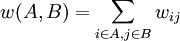
In the normalized cuts approach,^[1] for any cut $(S, \overline{S})$ in $G$ , $\operatorname{ncut}(S, \overline{S})$ measures the similarity between different parts, and $\operatorname{nassoc}(S, \overline{S})$ measures the total similarity of vertices in the same part.

Since $\operatorname{ncut}(S, \overline{S}) = 2 - \operatorname{nassoc}(S, \overline{S})$ , a cut $(S^{*}, {\overline{S}}^{*})$ that minimizes $\operatorname{ncut}(S, \overline{S})$ also maximizes $\operatorname{nassoc}(S, \overline{S})$ .

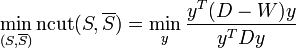
Computing a cut $(S^{*}, {\overline{S}}^{*})$ that minimizes $\operatorname{ncut}(S, \overline{S})$ is an NP-hard problem. However, we can find in polynomial time a cut $(S, \overline{S})$ of small normalized weight $\operatorname{ncut}(S, \overline{S})$ using spectral techniques.

The ncut algorithm

Let:

d(i) = \sum \limits_j w_{ij}

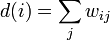
Also, let D be an $n \times n$ diagonal matrix with $d$ on the diagonal, and let $W$ be an $n \times n$ symmetric matrix with $w_{ij} = w_{ji}$ .

After some algebraic manipulations, we get:

\min \limits_{(S, \overline{S})} \operatorname{ncut}(S, \overline{S}) = \min \limits_y \frac{y^T (D - W) y}{y^T D y}

subject to the constraints:

$y_i \in \{1, -b \}$ , for some constant $-b$
$y^t D 1 = 0$

Minimizing 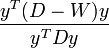$\frac{y^T (D - W) y}{y^T D y}$ subject to the constraints above is NP-hard. To make the problem tractable, we relax the constraints on $y$ , and allow it to take real values. The relaxed problem can be solved by solving the generalized eigenvalue problem $(D - W)y = \lambda D y$ for the second smallest generalized eigenvalue.

The partitioning algorithm:

Given a set of features, set up a weighted graph $G = (V, E)$ , compute the weight of each edge, and summarize the information in $D$ and $W$ .
Solve $(D - W)y = \lambda D y$ for eigenvectors with the smallest eigenvalues.
Use the eigenvector with the second smallest eigenvalue to bipartition the graph (e.g. grouping according to sign).
Decide if the current partition should be subdivided.
Recursively partition the segmented parts, if necessary.

Computational Complexity

Solving a standard eigenvalue problem for all eigenvectors (using the QR algorithm, for instance) takes $O(n^3)$ time. This is impractical for image segmentation applications where $n$ is the number of pixels in the image.

Since only one eigenvector, corresponding to the second smallest generalized eigenvalue, is used by the ncut algorithm, efficiency can be dramatically improved if the solve of the corresponding eigenvalue problem is performed in a matrix-free fashion, i.e., without explicitly manipulating with or even computing the matrix W, as, e.g., in the Lanczos algorithm. Matrix-free methods require only a function that performs a matrix-vector product for a given vector, on every iteration. For image segmentaion, the matrix W is typically sparse, with a number of nonzero entries $O(n)$ , so such a matrix-vector product takes $O(n)$ time.

For high-resolution images, the second eigenvalue is often ill-conditioned, leading to slow convergence of iterative eigenvalue solvers, such as the Lanczos algorithm.Preconditioning is a key technology accelerating the convergence, e.g., in the matrix-free LOBPCG method. Computing the eigenvector using an optimally preconditioned matrix-free method takes $O(n)$ time, which is the optimal complexity, since the eigenvector has $n$ components.

OBJ CUT

OBJ CUT^[2] is an efficient method that automatically segments an object. The OBJ CUT method is a generic method, and therefore it is applicable to any object category model. Given an image D containing an instance of a known object category, e.g. cows, the OBJ CUT algorithm computes a segmentation of the object, that is, it infers a set of labels m.

Let m be a set of binary labels, and let $\Theta$ be a shape parameter( $\Theta$ is a shape prior on the labels from a layered pictorial structure (LPS) model). An energy function $E(m, \Theta)$ is defined as follows.

E(m, \Theta) = \sum \phi_x(D|m_x) + \phi_x(m_x|\Theta) + \sum \Psi_{xy}(m_x, m_y) + \phi(D|m_x, m_y)

(1)

The term $\phi_x(D|m_x) + \phi_x(m_x|\Theta)$ is called a unary term, and the term $\Psi_{xy}(m_x, m_y) + \phi(D|m_x, m_y)$ is called a pairwise term. A unary term consists of the likelihood $\phi_x(D|m_x)$ based on color, and the unary potential $\phi_x(m_x|\Theta)$ based on the distance from $\Theta$ . A pairwise term consists of a prior $\Psi_{xy}(m_x, m_y)$ and a contrast term $\phi(D|m_x, m_y)$ .

The best labeling $m^{*}$ minimizes $\sum \limits_i w_i E(m, \Theta_i)$ , where $w_i$ is the weight of the parameter $\Theta_i$ .

m^{*} = \arg \min \limits_m \sum \limits_i w_i E(m, \Theta_i)

(2)

Algorithm

Given an image D, an object category is chosen, e.g. cows or horses.
The corresponding LPS model is matched to D to obtain the samples $\Theta_1, \cdots, \Theta_s$
The objective function given by equation (2) is determined by computing $E(m, \Theta_i)$ and using $w_i = g(\Theta_i|Z)$
The objective function is minimized using a single MINCUT operation to obtain the segmentation m.

Other approaches

Jigsaw approach^[3]
Image parsing ^[4]
Interleaved segmentation ^[5]
LOCUS ^[6]
LayoutCRF ^[7]
Minimum spanning tree-based segmentation

References

↑ Jianbo Shi and Jitendra Malik (1997): "Normalized Cuts and Image Segmentation", IEEE Conference on Computer Vision and Pattern Recognition, pp 731–737
↑ M. P. Kumar, P. H. S. Torr, and A. Zisserman. Obj cut. In Proceedings of IEEE Conference on Computer Vision and Pattern Recognition, San Diego, pages 18–25, 2005.
↑ E. Borenstein, S. Ullman: Class-specic, top-down segmentation. In Proceedings of the 7th European Conference on Computer Vision, Copenhagen, Denmark, pages 109–124, 2002.
↑ Z. Tu, X. Chen, A. L. Yuille, S. C. Zhu: Image Parsing: Unifying Segmentation, Detection, and Recognition. Toward Category-Level Object Recognition 2006: 545–576
↑ B. Leibe, A. Leonardis, B. Schiele: An Implicit Shape Model for Combined Object Categorization and Segmentation. Toward Category-Level Object Recognition 2006: 508–524
↑ J. Winn, N. Joijic. Locus: Learning object classes with unsupervised segmentation. In Proceedings of the IEEE International Conference on Computer Vision, Beijing, 2005.
↑ J. M. Winn, J. Shotton: The Layout Consistent Random Field for Recognizing and Segmenting Partially Occluded Objects. CVPR (1) 2006: 37–44

This article is issued from Wikipedia - version of the 5/5/2016. The text is available under the Creative Commons Attribution/Share Alike but additional terms may apply for the media files.