Scale analysis (mathematics)

Fit approximation

Concepts
Orders of approximation Scale analysis · Big O notation Curve fitting · False precision Significant figures
Other fundamentals
Approximation · Generalization error Taylor polynomial Scientific modelling

Scale analysis (or order-of-magnitude analysis) is a powerful tool used in the mathematical sciences for the simplification of equations with many terms. First the approximate magnitude of individual terms in the equations is determined. Then some negligibly small terms may be ignored.

Example: vertical momentum in synoptic-scale meteorology

Consider for example the momentum equation of the Navier–Stokes equations in the vertical coordinate direction of the atmosphere

{{\partial w} \over {\partial t}}+u{{\frac {\partial w}{\partial x}}}+v{{\frac {\partial w}{\partial y}}}+w{{\frac {\partial w}{\partial z}}}-{{\frac {u^{2}+v^{2}}{R}}}=-{{{\frac {1}{\varrho }}}{{\frac {\partial p}{\partial z}}}}-g+2{\Omega u\cos \varphi }+\nu \left({{\frac {\partial ^{2}w}{\partial x^{2}}}}+{{\frac {\partial ^{2}w}{\partial y^{2}}}}+{{\frac {\partial ^{2}w}{\partial z^{2}}}}\right),\qquad (1)

where R is Earth radius, Ω is frequency of rotation of the Earth, g is gravitational acceleration, φ is latitude, ρ is density of air and ν is kinematic viscosity of air (we can neglect turbulence in free atmosphere).

In synoptic scale we can expect horizontal velocities about U = 10¹ m.s⁻¹ and vertical about W = 10⁻² m.s⁻¹. Horizontal scale is L = 10⁶ m and vertical scale is H = 10⁴ m. Typical time scale is T = L/U = 10⁵ s. Pressure differences in troposphere are ΔP = 10⁴ Pa and density of air ρ = 10⁰ kg·m⁻³. Other physical properties are approximately:

R = 6.378 × 10⁶ m;

Ω = 7.292 × 10⁻⁵ rad·s^−1;

ν = 1.46 × 10⁻⁵ m²·s^−1;

g = 9.81 m·s^−2.

Estimates of the different terms in equation (1) can be made using their scales:

{\begin{aligned}{{\partial w} \over {\partial t}}&\sim {\frac {W}{T}}\\[1.2ex]u{{\frac {\partial w}{\partial x}}}&\sim U{\frac {W}{L}}&\qquad v{{\frac {\partial w}{\partial y}}}&\sim U{\frac {W}{L}}&\qquad w{{\frac {\partial w}{\partial z}}}&\sim W{\frac {W}{H}}\\[1.2ex]{{\frac {u^{2}}{R}}}&\sim {\frac {U^{2}}{R}}&\qquad {{\frac {v^{2}}{R}}}&\sim {\frac {U^{2}}{R}}\\[1.2ex]{\frac {1}{\varrho }}{\frac {\partial p}{\partial z}}&\sim {\frac {1}{\varrho }}{\frac {\Delta P}{H}}&\qquad \Omega u\cos \varphi &\sim \Omega U\\[1.2ex]\nu {\frac {\partial ^{2}w}{\partial x^{2}}}&\sim \nu {\frac {W}{L^{2}}}&\qquad \nu {\frac {\partial ^{2}w}{\partial y^{2}}}&\sim \nu {\frac {W}{L^{2}}}&\qquad \nu {\frac {\partial ^{2}w}{\partial z^{2}}}&\sim \nu {\frac {W}{H^{2}}}\end{aligned}}

Now we can introduce these scales and their values into equation (1):

{{\frac {10^{{-2}}}{10^{5}}}}+10{{\frac {10^{{-2}}}{10^{6}}}}+10{{\frac {10^{{-2}}}{10^{6}}}}+10^{{-2}}{{\frac {10^{{-2}}}{10^{4}}}}-{{\frac {10^{2}+10^{2}}{10^{6}}}}

=-{{{\frac {1}{1}}}{{\frac {10^{4}}{10^{4}}}}}-10+2\times 10^{{-4}}\times 10+10^{{-5}}\left({{\frac {10^{{-2}}}{10^{{12}}}}}+{{\frac {10^{{-2}}}{10^{{12}}}}}+{{\frac {10^{{-2}}}{10^{{8}}}}}\right).\qquad (2)

We can see that all terms — except the first and second on the right-hand side — are negligibly small. Thus we can simplify the vertical momentum equation to the hydrostatic equilibrium equation:

{{{\frac {1}{\varrho }}}{{\frac {\partial p}{\partial z}}}}=-g.\qquad (3)

Rules of scale analysis

Scale analysis is very useful and widely used tool for solving problems in the area of heat transfer and fluid mechanics, pressure-driven wall jet, separating flows behind backward-facing steps, jet diffusion flames, study of linear and non-linear dynamics. Scale analysis is recommended as the premier method for obtaining the most information per unit of intellectual effort, despite the fact that it is a precondition for good analysis in dimensionless form. The object of scale analysis is to use the basic principles of convective heat transfer to produce order-of-magnitude estimates for the quantities of interest. Scale analysis anticipates within a factor of order one when done properly, the expensive results produced by exact analyses. Scale analysis ruled as follows:

Rule1- First step in scale analysis is to define the domain of extent in which we apply scale analysis. Any scale analysis of a flow region that is not uniquely defined is not valid.

Rule2- One equation constitutes an equivalence between the scales of two dominant terms appearing in the equation. For example,

\rho c_{P}{{\partial T} \over {\partial t}}=k{\frac {\partial ^{2}T}{\partial x^{2}}}.

In the above example, the left-hand side could be of equal order of magnitude as the right-hand side.

Rule3- If in the sum of two terms given by

c=a+b

the order of magnitude of one term is greater than order of magnitude of the other term

O(a)>O(b)

then the order of magnitude of the sum is dictated by the dominant term

O(c)=O(a)

The same conclusion holds if we have the difference of two terms

c=a-b

Rule4- In the sum of two terms, if two terms are same order of magnitue,

c=a+b

O(a)=O(b)

then the sum is also of same order of magnitude:

O(a)\thicksim O(b)\thicksim O(c)

Rule5- In case of product of two terms

p=ab

the order of magnitude of the product is equal to the product of the orders of magnitude of the two factors

O(p)=O(a)O(b)

for ratios

r={\frac {a}{b}}

then

O(r)={\frac {O(a)}{O(b)}}

here O(a) represents the order of magnitude of a.

~ represents two terms are of same order of magnitude.

> represents greater than, in the sense of order-of-magnitude.

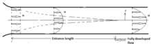
Developing flow in the entrance region of a parallel-plates duct

Scale analysis of fully developed flow

Consider the steady laminar flow of a viscous fluid inside a circular tube. Let the fluid enter with a uniform velocity over the flow across section. As the fluid moves down the tube a boundary layer of low-velocity fluid forms and grows on the surface because the fluid immediately adjacent to the surface have zero velocity. A particular and simplifying feature of viscous flow inside cylindrical tubes is the fact that the boundary layer must meet itself at the tube centerline, and the velocity distribution then establishes a fixed pattern that is invariant. Hydrodynamic entrance length as that part of the tube in which the momentum boundary layer grows and the velocity distribution changes with length. The fixed velocity distribution in the fully developed region is called fully developed velocity profile. The steady-state continuity and conservation of momentum equations in two-dimensional are

{{\partial u} \over {\partial x}}+{\frac {\partial v}{\partial y}}=0,\qquad (1)

u{{\partial u} \over {\partial x}}+v{\frac {\partial u}{\partial y}}=-{{\frac {1}{\varrho }}{\frac {\partial P}{\partial x}}}+\nu \left({\frac {\partial ^{2}u}{\partial x^{2}}}+{\frac {\partial ^{2}u}{\partial y^{2}}}\right),\qquad (2)

u{{\partial v} \over {\partial x}}+v{\frac {\partial v}{\partial y}}=-{{\frac {1}{\varrho }}{\frac {\partial P}{\partial y}}}+\nu \left({\frac {\partial ^{2}v}{\partial x^{2}}}+{\frac {\partial ^{2}v}{\partial y^{2}}}\right),\qquad (3)

These equations can be simplified by using scale analysis. At any point x ~ L in fully developed zone, we have y ~ D and u ~ U_∞. Now, from equation(1), the transverse velocity component in fully developed region simplified using scaling as

{\begin{aligned}v&\sim {\frac {U_{\infty }\delta }{L}}\qquad (4)\end{aligned}}

In fully developed region the section of the duct flow far from inlet such that scale of transverse velocity component v is negligible(L>>d).So, in fully developed flow limit, continuity equation requires

v=0,{{\partial u} \over {\partial x}}=0\qquad (5)

Based on equation(5), the y momentum equation eq3 reduces to

{{\partial P} \over {\partial y}}=0\qquad (6)

this means that P is function of x only. From this, the x momentum equation becomes

{{dP} \over {dx}}=\mu {{d^{2}u} \over {dy^{2}}}=constant\qquad (7)

Each term should be contant, because left side is function of x only and right is function of y. Solving equation(7) subject to the boundary condition

u=0,y=\pm {\frac {D}{2}}\qquad (8)

this results in the well-known Hagen–Poiseuille solution for fully developed flow between parallel plates.

u={\frac {3}{2}}U[1-{({\frac {y}{D/2}})}^{2}]\qquad (9)

U={\frac {D^{2}}{12\mu }}(-{\frac {dP}{dx}})\qquad (10)

where y is measured away from the center of the channel. The velocity is to be parabolic and is proportional to the pressure per unit duct length in the direction of the flow.

References

Barenblatt, G. I. (1996). Scaling, self-similarity, and intermediate asymptotics. Cambridge University Press. ISBN 0-521-43522-6.
Tennekes, H.; Lumley, John L. (1972). A first course in turbulence. MIT Press, Cambridge, Massachusetts. ISBN 0-262-20019-8.
Bejan, A. (2004). Convection Heat Transfer. John Wiley & sons. ISBN 978-81-265-0934-8.
Kays, W. M., Crawford M. E. (2012). Convective Heat and Mass Transfer. McGraw Hill Education(India). ISBN 978-1-25-902562-4.

External links

The Wikibook Partial Differential Equations has a page on the topic of: Scale Analysis

Scale analysis and Reynolds numbers

This article is issued from Wikipedia - version of the 11/5/2016. The text is available under the Creative Commons Attribution/Share Alike but additional terms may apply for the media files.