Savitzky–Golay filter

Animation showing smoothing being applied, passing through the data from left to right. The red line represents the local polynomial being used to fit a sub-set of the data. The smoothed values are shown as circles.

A Savitzky–Golay filter is a digital filter that can be applied to a set of digital data points for the purpose of smoothing the data, that is, to increase the signal-to-noise ratio without greatly distorting the signal. This is achieved, in a process known as convolution, by fitting successive sub-sets of adjacent data points with a low-degree polynomial by the method of linear least squares. When the data points are equally spaced, an analytical solution to the least-squares equations can be found, in the form of a single set of "convolution coefficients" that can be applied to all data sub-sets, to give estimates of the smoothed signal, (or derivatives of the smoothed signal) at the central point of each sub-set. The method, based on established mathematical procedures,^[1]^[2] was popularized by Abraham Savitzky and Marcel J. E. Golay who published tables of convolution coefficients for various polynomials and sub-set sizes in 1964.^[3]^[4] Some errors in the tables have been corrected.^[5] The method has been extended for the treatment of 2- and 3-dimensional data.

Savitzky and Golay's paper is one of the most widely cited papers in the journal Analytical Chemistry^[6] and is classed by that journal as one of its "10 seminal papers" saying "it can be argued that the dawn of the computer-controlled analytical instrument can be traced to this article".^[7]

Applications

The data consists of a set of n {x_j, y_j} points (j = 1, ..., n), where x is an independent variable and y_j is an observed value. They are treated with a set of m convolution coefficients, C_i, according to the expression

Y_{j}=\sum _{i=-{\tfrac {m-1}{2}}}^{\tfrac {m-1}{2}}C_{i}\,y_{j+i},\qquad {\frac {m+1}{2}}\leq j\leq n-{\frac {m-1}{2}}

It is easy to apply this formula in a spreadsheet. Selected convolution coefficients are shown in the tables, below. For example, for smoothing by a 5-point quadratic polynomial, m = 5, i = −2, −1, 0, 1, 2 and the jth smoothed data point, Y_j, is given by

Y_{j}={\frac {1}{35}}(-3y_{j-2}+12y_{j-1}+17y_{j}+12y_{j+1}-3y_{j+2})

where, C₋₂ = −3/35, C₋₁ = 12 / 35, etc. There are numerous applications of smoothing, which is performed primarily to make the data appear to be less noisy than it really is. The following are applications of numerical differentiation of data.^[8] Note When calculating the nth. derivative an additional scaling factor of $\frac{n!}{h^n}$ may be applied to all calculated data points to obtain absolute values (see expressions for $\frac{d^nY}{dx^n}$ , below, for details).

(1) Synthetic Lorentzian + noise (blue) and 1st. derivative (green)

(2) Titration curve (blue) for malonic acid and 2nd. derivative (green). The part in the light blue box is magnified 10 times

(3) Lorentzian on exponential baseline (blue) and 2nd. derivative (green)

(4) Sum of two Lorentzians (blue) and 2nd. derivative (green)

(5) 4th. derivative of the sum of two Lorentzians

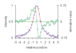
Location of maxima and minima in experimental data curves. This was the application that first motivated Savitzky.^[4] The first derivative of a function is zero at a maximum or minimum. The diagram shows data points belonging to a synthetic Lorentzian curve, with added noise (blue diamonds). Data are plotted on a scale of half width, relative to the peak maximum at zero. The smoothed curve (red line) and 1st. derivative (green) were calculated with 7-point cubic Savitzky–Golay filters. Linear interpolation of the first derivative values at positions either side of the zero-crossing gives the position of the peak maximum. 3rd. derivatives can also be used for this purpose.
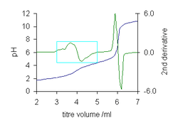
Location of an end-point in a titration curve. An end-point is an inflection point where the second derivative of the function is zero.^[9] The titration curve for malonic acid illustrates the power of the method. The first end-point at 4 ml is barely visible, but the second derivative allows its value to be easily determined by linear interpolation to find the zero crossing.
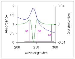
Baseline flattening. In analytical chemistry it is sometimes necessary to measure the height of an absorption band against a curved baseline.^[10] Because the curvature of the baseline is much less than the curvature of the absorption band, the second derivative effectively flattens the baseline. Three measures of the derivative height, which is proportional to the absorption band height, are the "peak-to-valley" distances h1 and h2, and the height from baseline, h3.^[11]
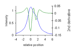
Resolution enhancement in spectroscopy. Bands in the second derivative of a spectroscopic curve are narrower than the bands in the spectrum: they have reduced half-width. This allows partially overlapping bands to be "resolved" into separate (negative) peaks.^[12] The diagram illustrates how this may be used also for chemical analysis, using measurement of "peak-to-valley" distances. In this case the valleys are a property of the 2nd. derivative of a Lorentzian. (x-axis position is relative to the position of the peak maximum on a scale of half width at half height).
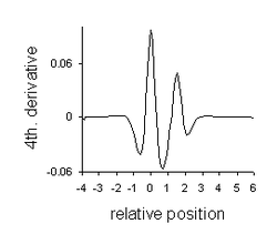
Resolution enhancement with 4th. derivative (positive peaks). The minima are a property of the 4th derivative of a Lorentzian.

Moving average

Main article: Moving average

A moving average filter is commonly used with time series data to smooth out short-term fluctuations and highlight longer-term trends or cycles. It is often used in technical analysis of financial data, like stock prices, returns or trading volumes. It is also used in economics to examine gross domestic product, employment or other macroeconomic time series.

An unweighted moving average filter is the simplest convolution filter. Each subset of the data set is fitted by a straight line. It was not included in the Savitzsky-Golay tables of convolution coefficients as all the coefficient values are simply equal to 1/m.

Derivation of convolution coefficients

When the data points are equally spaced, an analytical solution to the least-squares equations can be found.^[2] This solution forms the basis of the convolution method of numerical smoothing and differentiation. Suppose that the data consists of a set of n points (x_j, y_j) (j = 1, ..., n), where x is an independent variable and y_j is a datum value. A polynomial will be fitted by linear least squares to a set of m (an odd number) adjacent data points, each separated by an interval h. Firstly, a change of variable is made

z={{x-{\bar x}} \over h}

where ${{\bar x}}$ is the value of the central point. z takes the values ${\tfrac {1-m}{2}},\cdots ,0,\cdots ,{\tfrac {m-1}{2}}$ (e.g. m = 5 → z = −2, −1, 0, 1, 2).^{[note 1]} The polynomial, of degree k is defined as

Y=a_{0}+a_{1}z+a_{2}z^{2}\cdots +a_{k}z^{k}.

^{[note 2]}

The coefficients a₀, a₁ etc. are obtained by solving the normal equations (bold a represents a vector, bold J represents a matrix).

{{\mathbf {a}}}=\left({{{\mathbf {J}}}^{{{\mathbf {T}}}}{{\mathbf {J}}}}\right)^{{-{{\mathbf {1}}}}}{{\mathbf {J}}}^{{{\mathbf {T}}}}{{\mathbf {y}}}

The $i$ -th row of $\mathbf {J}$ has values $1,z_{i},z_{i}^{2},\dots$ .

For example, for a cubic polynomial fitted to 5 points, z= −2, −1, 0, 1, 2 the normal equations are solved as follows.

{\mathbf {J}}={\begin{pmatrix}1&-2&4&-8\\1&-1&1&-1\\1&0&0&0\\1&1&1&1\\1&2&4&8\end{pmatrix}}

\mathbf {J^{T}J} ={\begin{pmatrix}m&\sum z&\sum z^{2}&\sum z^{3}\\\sum z&\sum z^{2}&\sum z^{3}&\sum z^{4}\\\sum z^{2}&\sum z^{3}&\sum z^{4}&\sum z^{5}\\\sum z^{3}&\sum z^{4}&\sum z^{5}&\sum z^{6}\\\end{pmatrix}}={\begin{pmatrix}m&0&\sum z^{2}&0\\0&\sum z^{2}&0&\sum z^{4}\\\sum z^{2}&0&\sum z^{4}&0\\0&\sum z^{4}&0&\sum z^{6}\\\end{pmatrix}}={\begin{pmatrix}5&0&10&0\\0&10&0&34\\10&0&34&0\\0&34&0&130\\\end{pmatrix}}

Now, the normal equations can be factored into two separate sets of equations, by rearranging rows and columns, with

\mathbf {J^{T}J} _{even}={\begin{pmatrix}5&10\\10&34\\\end{pmatrix}}\quad \mathrm {and} \quad \mathbf {J^{T}J} _{odd}={\begin{pmatrix}10&34\\34&130\\\end{pmatrix}}

Expressions for the inverse of each of these matrices can be obtained using Cramer's rule

(\mathbf {J^{T}J} )_{\text{even}}^{-1}={1 \over 70}{\begin{pmatrix}34&-10\\-10&5\\\end{pmatrix}}\quad \mathrm {and} \quad (\mathbf {J^{T}J} )_{\text{odd}}^{-1}={1 \over 144}{\begin{pmatrix}130&-34\\-34&10\\\end{pmatrix}}

The normal equations become

{\begin{pmatrix}{a_{0}}\\{a_{2}}\\\end{pmatrix}}_{j}={1 \over 70}{\begin{pmatrix}34&-10\\-10&5\end{pmatrix}}{\begin{pmatrix}1&1&1&1&1\\4&1&0&1&4\\\end{pmatrix}}{\begin{pmatrix}y_{j-2}\\y_{j-1}\\y_{j}\\y_{j+1}\\y_{j+2}\end{pmatrix}}

and

{\begin{pmatrix}a_{1}\\a_{3}\\\end{pmatrix}}_{j}={1 \over 144}{\begin{pmatrix}130&-34\\-34&10\\\end{pmatrix}}{\begin{pmatrix}-2&-1&0&1&2\\-8&-1&0&1&8\\\end{pmatrix}}{\begin{pmatrix}y_{j-2}\\y_{j-1}\\y_{j}\\y_{j+1}\\y_{j+2}\\\end{pmatrix}}

Multiplying out and removing common factors,

{\begin{aligned}a_{0,j}&={1 \over 35}(-3y_{j-2}+12y_{j-1}+17y_{j}+12y_{j+1}-3y_{j+2})\\a_{1,j}&={1 \over 12}(y_{j-2}-8y_{j-1}+8y_{j+1}-y_{j+2})\\a_{2,j}&={1 \over 14}(2y_{j-2}-y_{j-1}-2y_{j}-y_{j+1}+2y_{j+2})\\a_{3,j}&={1 \over 12}(-y_{j-2}+2y_{j-1}-2y_{j+1}+y_{j+2})\end{aligned}}

The coefficients of y in these expressions are known as convolution coefficients. They are elements of the matrix

{\mathbf {C=(J^{T}J)^{{-1}}J^{T}}}

In general,

(C\otimes y)_{j}\ =Y_{j}=\sum _{i=-{\tfrac {m-1}{2}}}^{\tfrac {m-1}{2}}C_{i}\,y_{j+i},\qquad {\frac {m+1}{2}}\leq j\leq n-{\frac {m-1}{2}}

In matrix notation this example is written as

{\begin{pmatrix}Y_{3}\\Y_{4}\\Y_{5}\\\vdots \end{pmatrix}}={1 \over 35}{\begin{pmatrix}-3&12&17&12&-3&0&0&\cdots \\0&-3&12&17&12&-3&0&\cdots \\0&0&-3&12&17&12&-3&\cdots \\\vdots &\vdots &\vdots &\vdots &\vdots &\vdots &\vdots &\ddots \end{pmatrix}}{\begin{pmatrix}y_{1}\\y_{2}\\y_{3}\\y_{4}\\y_{5}\\y_{6}\\y_{7}\\\vdots \end{pmatrix}}

Tables of convolution coefficients, calculated in the same way for m up to 25, were published for the Savitzky–Golay smoothing filter in 1964,^[3]^[5] The value of the central point, z = 0, is obtained from a single set of coefficients, a₀ for smoothing, a₁ for 1st. derivative etc. The numerical derivatives are obtained by differentiating Y. This means that the derivatives are calculated for the smoothed data curve. For a cubic polynomial

{\begin{aligned}Y&=a_{0}+a_{1}z+a_{2}z^{2}+a_{3}z^{3}=a_{0}&{\text{ at }}z=0,x={\bar {x}}\\{\frac {dY}{dx}}&={\frac {1}{h}}\left({a_{1}+2a_{2}z+3a_{3}z^{2}}\right)={\frac {1}{h}}a_{1}&{\text{ at }}z=0,x={\bar {x}}\\{\frac {d^{2}Y}{dx^{2}}}&={\frac {1}{h^{2}}}\left({2a_{2}+6a_{3}z}\right)={\frac {2}{h^{2}}}a_{2}&{\text{ at }}z=0,x={\bar {x}}\\{\frac {d^{3}Y}{dx^{3}}}&={\frac {6}{h^{3}}}a_{3}\end{aligned}}

In general, polynomials of degree (0 and 1),^{[note 3]} (2 and 3), (4 and 5) etc. give the same coefficients for smoothing and even derivatives. Polynomials of degree (1 and 2), (3 and 4) etc. give the same coefficients for odd derivatives.

Algebraic expressions

It is not necessary always to use the Savitzky–Golay tables. The summations in the matrix J^TJ can be evaluated in closed form,

{\begin{aligned}\sum _{z=-{\frac {m-1}{2}}}^{\frac {m-1}{2}}z^{2}&={m(m^{2}-1) \over 12}\\\sum z^{4}&={m(m^{2}-1)(3m^{2}-7) \over 240}\\\sum z^{6}&={m(m^{2}-1)(3m^{4}-18m^{2}+31) \over 1344}\end{aligned}}

so that algebraic formulae can be derived for the convolution coefficients.^[13]^{[note 4]} Functions that are suitable for use with a curve that has an inflection point are:

Smoothing, polynomial degree 2,3 :

C_{{0i}}={\frac {{\left({3m^{2}-7-20i^{2}}\right)/4}}{{m\left({m^{2}-4}\right)/3}}};\quad {\frac {1-m}{2}}\leq i\leq {\frac {m-1}{2}}

(the range of values for i also applies to the expressions below)

1st derivative: polynomial degree 3,4

C_{{1i}}={\frac {{5\left({3m^{4}-18m^{2}+31}\right)i-28\left({3m^{2}-7}\right)i^{3}}}{{m\left({m^{2}-1}\right)\left({3m^{4}-39m^{2}+108}\right)/15}}}

2nd. derivative: polynomial degree 2,3

C_{2i} = \frac{{12mi^2 - m\left( {m^2 - 1} \right)}} {{m^2\left({m^2 - 1} \right) \left( {m^2 - 4} \right)/30}}

3rd. derivative: polynomial degree 3,4

C_{3i} = \frac{{ - \left( {3m^2 - 7} \right)i + 20i^3 }} {{m\left( {m^2 - 1} \right)\left( {3m^4 - 39m^2 + 108} \right)/2520}}

Simpler expressions that can be used with curves that don't have an inflection point are:

Smoothing, polynomial degree 0,1 (moving average):

C_{{0i}}={\frac {1}{m}}

1st derivative, polynomial degree 1,2:

C_{{1i}}={\frac {i}{m(m^{2}-1)/12}}

Higher derivatives can be obtained. For example, a fourth derivative can be obtained by performing two passes of a second derivative function.^[14]

Use of orthogonal polynomials

An alternative to fitting m data points by a simple polynomial in the subsidiary variable, z, is to use orthogonal polynomials.

Y=b_{0}P^{0}(z)+b_{1}P^{1}(z)\cdots +b_{k}P^{k}(z).

where P⁰ .. P^k is a set of mutually orthogonal polynomials of degree 0 .. k. Full details on how to obtain expressions for the orthogonal polynomials and the relationship between the coefficients b and a are given by Guest.^[2] Expressions for the convolution coefficients are easily obtained because the normal equations matrix, J^TJ, is a diagonal matrix as the product of any two orthogonal polynomials is zero by virtue of their mutual orthogonality. Therefore, each non-zero element of its inverse is simply the reciprocal the corresponding element in the normal equation matrix. The calculation is further simplified by using recursion to build orthogonal Gram polynomials. The whole calculation can be coded in a few lines of PASCAL, a computer language well-adapted for calculations involving recursion.^[15]

Treatment of first and last points

Savitzky–Golay filters are most commonly used to obtain the smoothed or derivative value at the central point, z = 0, using a single set of convolution coefficients. (m − 1)/2 points at the start and end of the series cannot be calculated using this process. Various strategies can be employed to avoid this inconvenience.

The data could be artificially extended by adding, in reverse order, copies of the first (m − 1)/2 points at the beginning and copies of the last (m − 1)/2 points at the end. For instance, with m = 5, two points are added at the start and end of the data y₁, ..., y_n.

y₃,y₂,y₁, ... ,y_n, y_n−1, y_n−2.

Looking again at the fitting polynomial, it is obvious that data can be calculated for all values of z by using all sets of convolution coefficients for a single polynomial, a₀ .. a_k.

For a cubic polynomial

{\begin{aligned}Y&=a_{0}+a_{1}z+a_{2}z^{2}+a_{3}z^{3}\\{\frac {dY}{dx}}&={\frac {1}{h}}\left({a_{1}+2a_{2}z+3a_{3}z^{2}}\right)\\{\frac {d^{2}Y}{dx^{2}}}&={\frac {1}{h^{2}}}\left({2a_{2}+6a_{3}z}\right)\\{\frac {d^{3}Y}{dx^{3}}}&={\frac {6}{h^{3}}}a_{3}\end{aligned}}

Convolution coefficients for the missing first and last points can also be easily obtained.^[15] This is also equivalent to fitting the first (m+1)/2 points with the same polynomial, and similarly for the last points.

Weighting the data

It is implicit in the above treatment that the data points are all given equal weight. Technically, the objective function

U=\sum _{i}w_{i}(Y_{i}-y_{i})^{2}

being minimized in the least-squares process has unit weights, w_i=1. When weights are not all the same the normal equations become

{\mathbf a}=\left({\mathbf {J^{T}W}}{\mathbf {J}}\right)^{{-1}}{\mathbf {J^{T}W}}{\mathbf {y}}\qquad W_{{i,i}}\neq 1

If the same set of diagonal weights is used for all data subsets, W = diag(w₁,w₂,...w_m), an analytical solution to the normal equations can be written down. For example, with a quadratic polynomial,

{\mathbf {J^{T}WJ}}={\begin{pmatrix}m\sum w_{i}&\sum w_{i}z_{i}&\sum w_{i}z_{i}^{2}\\\sum w_{i}z_{i}&\sum w_{i}z_{i}^{2}&\sum w_{i}z_{i}^{3}\\\sum w_{i}z_{i}^{2}&\sum w_{i}z_{i}^{3}&\sum w_{i}z_{i}^{4}\end{pmatrix}}

An explicit expression for the inverse of this matrix can be obtained using Cramer's rule. A set of convolution coefficients may then be derived as

{\mathbf C}=\left({\mathbf {J^{T}W}}{\mathbf {J}}\right)^{{-1}}{\mathbf {J^{T}W}}

Alternatively the coefficients, C, could be calculated in a spreadsheet, employing a built-in matrix inversion routine to obtain the inverse of the normal equations matrix. This set of coefficients, once calculated and stored, can be used with all calculations in which the same weighting scheme applies. A different set of coefficients is needed for each different weighting scheme.

Two-dimensional convolution coefficients

Two-dimensional smoothing and differentiation can also be applied to tables of data values, such as intensity values in a photographic image which is composed of a rectangular grid of pixels.^[16] ^[17] The trick is to transform part of the table into a row by a simple ordering of the indices of the pixels. Whereas the one-dimensional filter coefficients are found by fitting a polynomial in the subsidiary variable, z to a set of m data points, the two-dimensional coefficients are found by fitting a polynomial in subsidiary variables v and w to a set of m × m data points. The following example, for a bicubic polynomial and m = 5, illustrates the process, which parallels the process for the one dimensional case, above.^[18]

v={\frac {x-{\bar x}}{h(x)}};w={\frac {y-{\bar y}}{h(y)}}

Y=a_{{00}}+a_{{10}}v+a_{{01}}w+a_{{20}}v^{2}+a_{{11}}vw+a_{{02}}w^{2}+a_{{30}}v^{3}+a_{{21}}v^{2}w+a_{{12}}vw^{2}+a_{{03}}w^{3}

The square of 25 data values, $d 1 - d 25$

v w	−2	−1	0	1	2
−2	d₁	d₂	d₃	d₄	d₅
−1	d₆	d₇	d₈	d₉	d₁₀
0	d₁₁	d₁₂	d₁₃	d₁₄	d₁₅
1	d₁₆	d₁₇	d₁₈	d₁₉	d₂₀
2	d₂₁	d₂₂	d₂₃	d₂₄	d₂₅

becomes a vector when the rows are placed one after another.

d = (d₁ ... d₂₅)^T

The Jacobian has 10 columns, one for each of the parameters a₀₀ − a₀₃ and 25 rows, one for each pair of v and w values. Each row has the form

J_{{\text{row}}}=1\ v\ w\ v^{2}\ vw\ w^{2}\ v^{3}\ v^{2}w\ vw^{2}\ w^{3}

The convolution coefficients are calculated as

{\mathbf {C}}=\left({\mathbf {J}}^{T}{\mathbf {J}}\right)^{{-1}}{\mathbf {J}}^{T}

The first row of C contains 25 convolution coefficients which can be multiplied with the 25 data values to provide a smoothed value for the central data point (13) of the 25.

A Matlab^[19] routine for computing the coefficients is available. 3-dimensional filters can be obtained with a similar procedure.^[16]^[20]

Some properties of convolution

The sum of convolution coefficients for smoothing is equal to one. The sum of coefficients for odd derivatives is zero.^[21]
The sum of squared convolution coefficients for smoothing is equal to the value of the central coefficient.^[22]
Smoothing of a function leaves the area under the function unchanged.^[21]
Convolution of a symmetric function with even-derivative coefficients conserves the centre of symmetry.^[21]
Properties of derivative filters.^[23]

Signal distortion and noise reduction

It is inevitable that the signal will be distorted in the convolution process. From property 3 above, when data which has a peak is smoothed the peak height will be reduced and the half-width will be increased. Both the extent of the distortion and S/N (signal-to-noise ratio) improvement:

decrease as the degree of the polynomial increases
increase as the width, m of the convolution function increases

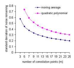
Effect of smoothing on data points with uncorrelated noise of unit standard deviation

For example, If the noise in all data points is uncorrelated and has a constant standard deviation, σ, the standard deviation on the noise will be decreased by convolution with an m-point smoothing function to^[22]^{[note 5]}

polynomial degree 0 or 1:

{\sqrt {{1 \over m}}}\sigma

(moving average)

polynomial degree 2 or 3:

{\sqrt {{\frac {3(3m^{2}-7)}{4m(m^{2}-4)}}}}\sigma

These functions are shown in the plot at the right. For example, with a 9-point linear function (moving average) two thirds of the noise is removed and with a 9-point quadratic/cubic smoothing function only about half the noise is removed. Most of the noise remaining is low-frequency noise(see Frequency characteristics of convolution filters, below).

Although the moving average function gives the best noise reduction it is unsuitable for smoothing data which has curvature over m points. A quadratic filter function is unsuitable for getting a derivative of a data curve with an inflection point because a quadratic polynomial does not have one. The optimal choice of polynomial order and number of convolution coefficients will be a compromise between noise reduction and distortion.^[24]

Multipass filters

One way to mitigate distortion and improve noise removal is to use a filter of smaller width and perform more than one convolution with it. For two passes of the same filter this is equivalent to one pass of a filter obtained by convolution of the original filter with itself.^[25] For example, 2 passes of the filter with coefficients (1/3, 1/3, 1/3) is equivalent to 1 pass of the filter with coefficients (1/9, 2/9, 3/9, 2/9, 1/9).

The disadvantage of multipassing is that the equivalent filter width for n passes of an m-point function is n(m − 1) + 1 so multipassing is subject to greater end-effects. Nevertheless, multipassing has been used to great advantage. For instance, some 40–80 passes on data with a signal-to-noise ratio of only 5 gave useful results.^[26] The noise reduction formulae given above do not apply because correlation between calculated data points increases with each pass.

Frequency characteristics of convolution filters

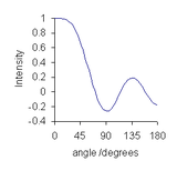
Fourier transform of the 9-point quadratic/cubic smoothing function

Convolution maps to multiplication in the Fourier co-domain. The discrete Fourier transform of a convolution filter is a real-valued function which can be represented as

FT(\theta )=\sum _{j={\tfrac {1-m}{2}}}^{\tfrac {m-1}{2}}C_{j}\cos(j\theta )

θ runs from 0 to 180 degrees, after which the function merely repeats itself. The plot for a 9-point quadratic/cubic smoothing function is typical. At very low angle, the plot is almost flat, meaning that low-frequency components of the data will be virtually unchanged by the smoothing operation. As the angle increases the value decreases so that higher frequency components are more and more attenuated. This shows that the convolution filter can be described as a low-pass filter: the noise that is removed is primarily high-frequency noise and low-frequency noise passes through the filter.^[27] Some high-frequency noise components are attenuated more than others, as shown by undulations in the Fourier transform at large angles. This can give rise to small oscillations in the smoothed data.^[28]

Convolution and correlation

Convolution affects the correlation between errors in the data. The effect of convolution can be expressed as a linear transformation.

Y_{j}\ =\sum _{i=-{\frac {m-1}{2}}}^{\frac {m-1}{2}}C_{i}\,y_{j+i}

By the law of error propagation, the variance-covariance matrix of the data, A will be transformed into B according to

{\mathbf B}={\mathbf C}{\mathbf A}{\mathbf C}^{T}

To see how this applies in practice, consider the effect of a 3-point moving average on the first three calculated points, $Y 2 - Y 4$ , assuming that the data points have equal variance and that there is no correlation between them. A will be an identity matrix multiplied by a constant, σ², the variance at each point.

\mathbf {B} ={\sigma ^{2} \over 9}{\begin{pmatrix}1&1&1&0&0\\0&1&1&1&0\\0&0&1&1&1\\\end{pmatrix}}{\begin{pmatrix}1&0&0&0&0\\0&1&0&0&0\\0&0&1&0&0\\0&0&0&1&0\\0&0&0&0&1\\\end{pmatrix}}{\begin{pmatrix}1&0&0\\1&1&0\\1&1&1\\0&1&1\\0&0&1\\\end{pmatrix}}={\sigma ^{2} \over 9}{\begin{pmatrix}3&2&1\\2&3&2\\1&2&3\\\end{pmatrix}}

In this case the correlation coefficients,

\rho _{ij}={\frac {B_{ij}}{\sqrt {B_{ii}B_{jj}}}},\ (i\neq j)

between calculated points i and j will be

\rho _{{i,i+1}}={2 \over 3}=0.66

\rho _{{i,i+2}}={1 \over 3}=0.33

In general, the calculated values are correlated even when the observed values are not correlated. The correlation extends over $m - 1$ calculated points at a time.^[29]

Multipass filters

To illustrate the effect of multipassing on the noise and correlation of a set of data, consider the effects of a second pass of a 3-point moving average filter. For the second pass^{[note 6]}

\mathbf {CBC^{T}} ={\sigma ^{2} \over 81}{\begin{pmatrix}1&1&1&0&0\\0&1&1&1&0\\0&0&1&1&1\\\end{pmatrix}}{\begin{pmatrix}3&2&1&0&0\\2&3&2&0&0\\1&2&3&0&0\\0&0&0&0&0\\0&0&0&0&0\\\end{pmatrix}}{\begin{pmatrix}1&0&0\\1&1&0\\1&1&1\\0&1&1\\0&0&1\\\end{pmatrix}}={\sigma ^{2} \over 81}{\begin{pmatrix}19&16&10&4&1\\16&19&16&10&4\\10&16&19&16&10\\4&10&16&19&16\\1&4&10&16&19\end{pmatrix}}

After two passes, the standard deviation of the central point has decreased to ${\sqrt {\tfrac {19}{81}}}\sigma =0.48\sigma$ , compared to 0.58σ for one pass. The noise reduction is a little less than would be obtained with one pass of a 5-point moving average which, under the same conditions, would result in the smoothed points having the smaller standard deviation of 0.45σ.

Correlation now extends over a span of 4 sequential points with correlation coefficients

\rho _{{i,i+1}}={16 \over 19}=0.84,\rho _{{i,i+2}}={10 \over 19}=0.53,\rho _{{i,i+3}}={4 \over 19}=0.21,\rho _{{i,i+4}}={1 \over 19}=0.05

The advantage obtained by performing two passes with the narrower smoothing function is that it introduces less distortion into the calculated data.

Appendix

Tables of selected convolution coefficients

Consider a set of data points $(x_{j},y_{j})_{1\leq j\leq n}$ . The Savitzky–Golay tables refer to the case that the step $x_{j}-x_{j-1}$ is constant, h. Examples of the use of the so-called convolution coefficients, with a cubic polynomial and a window size, m, of 5 points are as follows.

Smoothing: $Y_{j}={\frac {1}{35}}(-3\times y_{{j-2}}+12\times y_{{j-1}}+17\times y_{j}+12\times y_{{j+1}}-3\times y_{{j+2}})$ ;
1st derivative: $Y'_{j}={\frac {1}{12h}}(1\times y_{{j-2}}-8\times y_{{j-1}}+0\times y_{j}+8\times y_{{j+1}}-1\times y_{{j+2}})$ ;
2nd derivative: $Y''_j = \frac{2}{7h^2} (2 \times y_{j - 2} - 1 \times y_{j - 1} - 2 \times y_j - 1 \times y_{j + 1} + 2 \times y_{j + 2})$ .

Selected values of the convolution coefficients for polynomials of degree 1,2,3, 4 and 5 are given in the following tables. The values were calculated using the PASCAL code provided in Gorry.^[15]

Coefficients for smoothing
Degree	2/3 (quadratic/cubic)			4/5 (quartic/quintic)
Window size	5	7	9	7	9
−4			−21		15
−3		−2	14	5	−55
−2	−3	3	39	−30	30
−1	12	6	54	75	135
0	17	7	59	131	179
1	12	6	54	75	135
2	−3	3	39	−30	30
3		−2	14	5	−55
4			−21		15
Normalisation	35	21	231	231	429

Coefficients for 1st derivative
Degree	1/2 (linear/quadratic)				3/4 (cubic/quartic)
Window size	3	5	7	9	5	7	9
−4				−4			86
−3			−3	−3		22	−142
−2		−2	−2	−2	1	−67	−193
−1	-1	−1	−1	−1	−8	−58	−126
0	0	0	0	0	0	0	0
1	1	1	1	1	8	58	126
2		2	2	2	−1	67	193
3			3	3		−22	142
4				4			−86
Normalisation	2	10	28	60	12	252	1,188

Coefficients for 2nd derivative
Degree	2/3 (quadratic/cubic)			4/5 (quartic/quintic)
Window size	5	7	9	5	7	9
−4			28			−126
−3		5	7		−13	371
−2	2	0	−8	−1	67	151
−1	−1	−3	−17	16	−19	−211
0	−2	−4	−20	−30	−70	−370
1	−1	−3	−17	16	−19	−211
2	2	0	−8	−1	67	151
3		5	7		−13	371
4			28			−126
Normalisation	7	42	462	12	132	1716

Coefficients for 3rd derivative
Degree	3/4 (cubic/quartic)			5/6 (quintic/sextic)
Window size	5	7	9	7	9
−4			−14		100
−3		−1	7	1	−457
−2	−1	1	13	−8	256
−1	2	1	9	13	459
0	0	0	0	0	0
1	−2	−1	−9	−13	−459
2	1	−1	−13	8	−256
3		1	−7	−1	457
4			14		−100
Normalisation	2	6	198	8	1144

Coefficients for 4th derivative
Degree	4/5 (quartic/quintic)
Window size	7	9
−4		14
−3	3	−21
−2	−7	−11
−1	1	9
0	6	18
1	1	9
2	-7	−11
3	3	−21
4		14
Normalisation	11	143

Notes

↑ With even values of m, z will run from 1 − m to m − 1 in steps of 2
↑ The simple moving average is a special case with k = 0, Y = a₀. In this case all convolution coefficients are equal to 1/m.
↑ Smoothing using the moving average is equivalent, with equally spaced points, to local fitting with a (sloping) straight line
↑ The expressions given here are different from those of Madden, which are given in terms of the variable m' = (m − 1)/2.
↑ The expressions under the square root sign are the same as the expression for the convolution coefficient with z=0
↑ The same result is obtained with one pass of the equivalent filter with coefficients (1/9, 2/9, 3/9, 2/9, 1/9) and an identity variance-covariance matrix

References

↑ Whittaker, E.T; Robinson, G (1924). The Calculus Of Observations. Blackie & Son. pp. 291–6. OCLC 1187948. . "Graduation Formulae obtained by fitting a Polynomial."
1 2 3 Guest, P.G. (2012) [1961]. "Ch. 7: Estimation of Polynomial Coefficients". Numerical Methods of Curve Fitting. Cambridge University Press. pp. 147–. ISBN 978-1-107-64695-7.
1 2 Savitzky, A.; Golay, M.J.E. (1964). "Smoothing and Differentiation of Data by Simplified Least Squares Procedures". Analytical Chemistry. 36 (8): 1627–39. doi:10.1021/ac60214a047.
1 2 Savitzky, Abraham (1989). "A Historic Collaboration". Analytical Chemistry. 61 (15): 921A–3A. doi:10.1021/ac00190a744.
1 2 Steinier, Jean; Termonia, Yves; Deltour, Jules (1972). "Smoothing and differentiation of data by simplified least square procedure". Analytical Chemistry. 44 (11): 1906–9. doi:10.1021/ac60319a045.
↑ Larive, Cynthia K.; Sweedler, Jonathan V. (2013). "Celebrating the 75th Anniversary of the ACS Division of Analytical Chemistry: A Special Collection of the Most Highly Cited Analytical Chemistry Papers Published between 1938 and 2012". Analytical Chemistry. 85 (0): 4201–2. doi:10.1021/ac401048d.
↑ Riordon, James; Zubritsky, Elizabeth; Newman, Alan (2000). "Top 10 Articles". Analytical Chemistry. 72 (9): 24 A–329 A. doi:10.1021/ac002801q.
↑ Talsky, Gerhard. Derivative Spectrophotometry. Wiley. ISBN 3527282947.
↑ Abbaspour, Abdolkarim; Khajehzadeha, Abdolreza (2012). "End point detection of precipitation titration by scanometry method without using indicator". Anal. Methods. 4: 923–932. doi:10.1039/C2AY05492B.
↑ Li, N; Li, XY; Zou, XZ; Lin, LR; Li, YQ (2011). "A novel baseline-correction method for standard addition based derivative spectra and its application to quantitative analysis of benzo(a)pyrene in vegetable oil samples.". Analyst. 136 (13): 2802–10. doi:10.1039/c0an00751j.
↑ Dixit, L.; Ram, S. (1985). "Quantitative Analysis by Derivative Electronic Spectroscopy". Applied Spectroscopy Reviews. 21 (4): 311–418. doi:10.1080/05704928508060434.
↑ Giese, Arthur T.; French, C. Stacey (1955). "The Analysis of Overlapping Spectral Absorption Bands by Derivative Spectrophotometry". Appl. Spectrosc. 9 (2): 78–96. doi:10.1366/000370255774634089.
↑ Madden, Hannibal H. (1978). "Comments on the Savitzky–Golay convolution method for least-squares-fit smoothing and differentiation of digital data" (PDF). Anal. Chem. 50 (9): 1383–6. doi:10.1021/ac50031a048.
↑ Gans 1992, pp. 153–7, "Repeated smoothing and differentiation"
1 2 3 A., Gorry (1990). "General least-squares smoothing and differentiation by the convolution (Savitzky–Golay) method". Analytical Chemistry. 62 (6): 570–3. doi:10.1021/ac00205a007.
1 2 Thornley, David J. Anisotropic Multidimensional Savitzky Golay kernels for Smoothing, Differentiation and Reconstruction (PDF) (Technical report). Imperial College Department of Computing. 2066/8.
↑ Ratzlaff, Kenneth L.; Johnson, Jean T. (1989). "Computation of two-dimensional polynomial least-squares convolution smoothing integers". Anal. Chem. 61 (11): 1303–5. doi:10.1021/ac00186a026.
↑ Krumm, John. "Savitzky–Golay filters for 2D Images". Microsoft Research, Redmond.
↑ Krumm, John. "Compute Savitzky−Golay coefficients". Microsoft Research, Redmond.
↑ Bagge Carlson, Fredrik. "Polynomial reconstruction of 3D sampled curves using auxiliary surface data". IEEE.
1 2 3 Gans & 1992 Appendix 7
1 2 Ziegler, Horst (1981). "Properties of Digital Smoothing Polynomial (DISPO) Filters". Applied Spectroscopy. 35 (1): 88–92. doi:10.1366/0003702814731798.
↑ Luo, Jianwen; Ying, Kui; He, Ping; Bai, Jing (2005). "Properties of Savitzky–Golay digital differentiators" (PDF). Digital Signal Processing. 15: 122–136. doi:10.1016/j.dsp.2004.09.008.
↑ Gans, Peter; Gill, J. Bernard (1983). "Examination of the Convolution Method for Numerical Smoothing and Differentiation of Spectroscopic Data in Theory and in Practice". Applied Spectroscopy. 37 (6): 515–520. doi:10.1366/0003702834634712.
↑ Gans 1992, pp. 153
↑ Procter, Andrew; Sherwood, Peter M.A. (1980). "Smoothing of digital x-ray photoelectron spectra by an extended sliding least-squares approach". Anal. Chem. 52 (14): 2315–21. doi:10.1021/ac50064a018.
↑ Gans 1992, pp. 207
↑ Bromba, Manfred U.A; Ziegler, Horst (1981). "Application hints for Savitzky–Golay digital smoothing filters". Anal. Chem. 53 (11): 1583–6. doi:10.1021/ac00234a011.
↑ Gans 1992, pp. 157

Gans, Peter (1992). Data fitting in the chemical sciences: By the method of least squares. ISBN 9780471934127.

External links

Wikimedia Commons has media related to Savitzky–Golay filter.

Savitzky–Golay filter in Fundamentals of Statistics

This article is issued from Wikipedia - version of the 11/21/2016. The text is available under the Creative Commons Attribution/Share Alike but additional terms may apply for the media files.

Savitzky–Golay filter

Applications

Moving average

Derivation of convolution coefficients

Algebraic expressions

Use of orthogonal polynomials

Treatment of first and last points

Weighting the data

Two-dimensional convolution coefficients

Some properties of convolution

Signal distortion and noise reduction

Multipass filters

Frequency characteristics of convolution filters

Convolution and correlation

Multipass filters

See also

Appendix

Tables of selected convolution coefficients

Notes

References

External links