Rindler coordinates

In relativistic physics, the Rindler coordinate chart is an important and useful coordinate chart representing part of flat spacetime, also called the Minkowski vacuum. The Rindler coordinate system or frame describes a uniformly accelerating frame of reference in Minkowski space. In special relativity, a uniformly accelerating particle undergoes hyperbolic motion. For each such particle, a Rindler frame can be chosen in which it is at rest.

The Rindler chart is named after Wolfgang Rindler who popularised its use, although it was already "well known" in 1935, according to a paper by Albert Einstein and Nathan Rosen.^[1]

Relation to Cartesian chart

Rindler chart, for g=1, plotted on a Minkowski diagram. The dashed lines are the Rindler horizons

To obtain the Rindler chart, start with the Cartesian chart (an inertial frame) with the metric (c=1 is assumed)

ds^{2}=-dT^{2}+dX^{2}+dY^{2}+dZ^{2},\;\forall T,X,Y,Z\,.

In the region $\scriptstyle 0 \,<\, X \,<\, \infty,\; -X \,<\, T \,<\, X$ , which is often called the Rindler wedge, if g represents the proper acceleration (along the hyperbola x=1) of the Rindler observer whose proper time is defined to be equal to Rindler coordinate time (see below), the new chart is defined using the coordinate transformation

t={\frac {1}{g}}\operatorname {arctanh}\left({\frac {T}{X}}\right),\;x={\sqrt {X^{2}-T^{2}}},\;y=Y,\;z=Z\,.

The inverse transformation is

T=x\,\sinh(gt),\;X=x\,\cosh(gt),\;Y=y,\;Z=z\,.

In the Rindler chart, the Minkowski line element becomes

ds^{2}=-g^{2}x^{2}dt^{2}+dx^{2}+dy^{2}+dz^{2},\;\forall x>0,\forall t,y,z\,.

A Rindler observer is defined as an observer that is "at rest" in Rindler coordinates, i.e., maintaining constant x, y, z and only varying t as time passes. To maintain this world line, the observer must accelerate with a constant proper acceleration, with Rindler observers closer to x=0 (the Rindler horizon) having greater proper acceleration. All the Rindler observers are instantaneously at rest at time T=0 in the inertial frame, and at this time a Rindler observer with proper acceleration g_i will be at position X = 1/g_i (really X = c²/g_i, but we assume units where c=1), which is also that observer's constant distance from the Rindler horizon in Rindler coordinates. If all Rindler observers set their clocks to zero at T=0, then when defining a Rindler coordinate system we have a choice of which Rindler observer's proper time will be equal to the coordinate time t in Rindler coordinates, and this observer's proper acceleration defines the value of g above (for other Rindler observers at different distances from the Rindler horizon, the coordinate time will equal some constant multiple of their own proper time).^[2] It is a common convention to define the Rindler coordinate system so that the Rindler observer whose proper time matches coordinate time is the one who has proper acceleration g=1, so that g can be eliminated from the equations.

The above equation,

t = \frac{1}{g} \operatorname{arctanh}\left(\frac{T}{X}\right),\; x= \sqrt{X^2-T^2},\; y = Y,\; z = Z

has been simplified for c=1. The unsimplified equation is more convenient for finding the Rindler Horizon distance, given an acceleration g.

\begin{align} t &= \frac{c}{g} \operatorname{arctanh}\left (\frac{c T}{X}\right) \;\overset {X \,\gg\, cT}\approx\; \frac{c^2 T}{g X}\\ X &\approx \frac{c^2 T}{g t} \;\overset{T \,\approx\, t}\approx\; \frac{c^2 }{g} \end{align}

The remainder of the article will follow the convention of setting both g=1 and c=1, so units for X and x will be 1 unit = c^2/g = 1. Be mindful that setting g=1 light-second/second² is very different from setting g=1 light-year/year^2. Even if we pick units where c=1, the magnitude of the proper acceleration g will depend on our choice of units: for example, if we use units of light-years for distance, (X or x) and years for time, (T or t), this would mean g = 1 light year/year², equal to about 9.5 meters/second², while if we use units of light-seconds for distance, (X or x), and seconds for time, (T or t), this would mean g = 1 light-second/second², or 299792458 meters/second²).

The Rindler observers

In the new chart, it is natural to take the coframe field

d\sigma^0 = -x \, dt,\;\; d\sigma^1 = dx,\;\; d\sigma^2 = dy,\;\; d\sigma^3 = dz

which has the dual frame field

\vec{e}_0 = \frac{1}{x}\partial_t,\;\; \vec{e}_1 = \partial_x,\;\; \vec{e}_2 = \partial_y,\;\; \vec{e}_3 = \partial_z

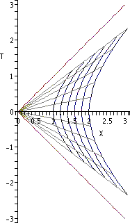
This defines a local Lorentz frame in the tangent space at each event (in the region covered by our Rindler chart, namely the Rindler wedge). The integral curves of the timelike unit vector field $\scriptstyle\vec{e}_0$ give a timelike congruence, consisting of the world lines of a family of observers called the Rindler observers. In the Rindler chart, these world lines appear as the vertical coordinate lines $\scriptstyle x \;=\; x_0,\; y \;=\; y_0,\; z \;=\; z_0$ . Using the coordinate transformation above, we find that these correspond to hyperbolic arcs in the original Cartesian chart.

As with any timelike congruence in any Lorentzian manifold, this congruence has a kinematic decomposition (see Raychaudhuri equation). In this case, the expansion and vorticity of the congruence of Rindler observers vanish. The vanishing of the expansion tensor implies that each of our observers maintains constant distance to his neighbors. The vanishing of the vorticity tensor implies that the world lines of our observers are not twisting about each other; this is a kind of local absence of "swirling".

The acceleration vector of each observer is given by the covariant derivative

\nabla_{\vec{e}_0} \vec{e}_0 = \frac{1}{x}\vec{e}_1

That is, each Rindler observer is accelerating in the $\scriptstyle\partial_x$ direction. Individually speaking, each observer is in fact accelerating with constant magnitude in this direction, so their world lines are the Lorentzian analogs of circles, which are the curves of constant path curvature in the Euclidean geometry.

Because the Rindler observers are vorticity-free, they are also hypersurface orthogonal. The orthogonal spatial hyperslices are $\scriptstyle t \;=\; t_0$ ; these appear as horizontal half-planes in the Rindler chart and as half-planes through $\scriptstyle T \;=\; X \;=\; 0$ in the Cartesian chart (see the figure above). Setting $\scriptstyle dt \;=\; 0$ in the line element, we see that these have the ordinary Euclidean geometry, $\scriptstyle d\sigma^2 \;=\; dx^2 \,+\, dy^2 \,+\, dz^2,\; \forall x\,>\,0,\; \forall y,\, z$ . Thus, the spatial coordinates in the Rindler chart have a very simple interpretation consistent with the claim that the Rindler observers are mutually stationary. We will return to this rigidity property of the Rindler observers a bit later in this article.

A "paradoxical" property

Note that Rindler observers with smaller constant x coordinate are accelerating harder to keep up! This may seem surprising because in Newtonian physics, observers who maintain constant relative distance must share the same acceleration. But in relativistic physics, we see that the trailing endpoint of a rod which is accelerated by some external force (parallel to its symmetry axis) must accelerate a bit harder than the leading endpoint, or else it must ultimately break. This is a manifestation of Lorentz contraction. As the rod accelerates its velocity increases and its length decreases. Since it is getting shorter, the back end must accelerate harder than the front. Another way to look at it is: the back end must achieve the same change in velocity in a shorter period of time. This leads to a differential equation showing, that at some distance, the acceleration of the trailing end diverges, resulting in the Rindler horizon.

This phenomenon is the basis of a well known "paradox", Bell's spaceship paradox. However, it is a simple consequence of relativistic kinematics. One way to see this is to observe that the magnitude of the acceleration vector is just the path curvature of the corresponding world line. But the world lines of our Rindler observers are the analogs of a family of concentric circles in the Euclidean plane, so we are simply dealing with the Lorentzian analog of a fact familiar to speed skaters: in a family of concentric circles, inner circles must bend faster (per unit arc length) than the outer ones.

Minkowski observers

It is worthwhile to also introduce an alternative frame, given in the Minkowski chart by the natural choice

\vec{f}_0 = \partial_T, \; \vec{f}_1 = \partial_X, \; \vec{f}_2 = \partial_Y, \; \vec{f}_3 = \partial_Z

Transforming these vector fields using the coordinate transformation given above, we find that in the Rindler chart (in the Rinder wedge) this frame becomes

\begin{align} \vec{f}_0 &= \frac{1}{x}\cosh(t) \, \partial_t - \sinh(t) \, \partial_x\\ \vec{f}_1 &= -\frac{1}{x}\sinh(t) \, \partial_t + \cosh(t) \, \partial_x\\ \vec{f}_2 &= \partial_y, \; \vec{f}_3 = \partial_z \end{align}

Computing the kinematic decomposition of the timelike congruence defined by the timelike unit vector field $\scriptstyle\vec{f}_0$ , we find that the expansion and vorticity again vanishes, and in addition the acceleration vector vanishes, $\scriptstyle\nabla_{\vec{f}_0} \vec{f}_0 \;=\; 0$ . In other words, this is a geodesic congruence; the corresponding observers are in a state of inertial motion. In the original Cartesian chart, these observers, whom we will call Minkowski observers, are at rest.

In the Rindler chart, the world lines of the Minkowski observers appear as hyperbolic secant curves asymptotic to the coordinate plane $\scriptstyle x \;=\; 0$ . Specifically, in Rindler coordinates, the world line of the Minkowski observer passing through the event $\scriptstyle t \;=\; t_0,\; x \;=\; x_0,\; y \;=\; y_0,\; z \;=\; z_0$ is

\begin{align} t &= \operatorname{arctanh}\left(\frac{s}{x_0}\right),\; -x_0 < s < x_0\\ x &= \sqrt{x_0^2-s^2},\; -x_0 < s < x_0\\ y &= y_0\\ z &= z_0 \end{align}

where $\scriptstyle s$ is the proper time of this Minkowski observer. Note that only a small portion of his history is covered by the Rindler chart! This shows explicitly why the Rindler chart is not geodesically complete; timelike geodesics run outside the region covered by the chart in finite proper time. Of course, we already knew that the Rindler chart cannot be geodesically complete, because it covers only a portion of the original Cartesian chart, which is a geodesically complete chart.

In the case depicted in the figure, $\scriptstyle x_0 \;=\; 1$ and we have drawn (correctly scaled and boosted) the light cones at $\scriptstyle s \,\in\, \left\{-\frac{1}{2},\; 0,\; \frac{1}{2}\right\}$ .

The Rindler horizon

The Rindler coordinate chart has a coordinate singularity at x = 0, where the metric tensor (expressed in the Rindler coordinates) has vanishing determinant. This happens because as x → 0 the acceleration of the Rindler observers diverges. As we can see from the figure illustrating the Rindler wedge, the locus x = 0 in the Rindler chart corresponds to the locus T² = X², X > 0 in the Cartesian chart, which consists of two null half-planes, each ruled by a null geodesic congruence.

For the moment, we simply consider the Rindler horizon as the boundary of the Rindler coordinates. If we consider the set of accelerating observers who have a constant position in Rindler coordinates, none of them can ever receive light signals from events with T ≥ X (on the diagram, these would be events on or to the left of the line T = X which the upper red horizon lies along; these observers could however receive signals from events with T ≥ X if they stopped their acceleration and crossed this line themselves) nor could they have ever sent signals to events with T ≤ −X (events on or to the left of the line T = −X which the lower red horizon lies along; those events lie outside all future light cones of their past world line). Also, if we consider members of this set of accelerating observers closer and closer to the horizon, in the limit as the distance to the horizon approaches zero, the constant proper acceleration experienced by an observer at this distance (which would also be the G-force experienced by such an observer) would approach infinity. Both of these facts would also be true if we were considering a set of observers hovering outside the event horizon of a black hole, each observer hovering at a constant radius in Schwarzschild coordinates. In fact, in the close neighborhood of a black hole, the geometry close to the event horizon can be described in Rindler coordinates. Hawking radiation in the case of an accelerating frame is referred to as Unruh radiation. The connection is the equivalence of acceleration with gravitation.^[3]

Geodesics

The geodesic equations in the Rindler chart are easily obtained from the geodesic Lagrangian; they are

\ddot{t} + \frac{2}{x} \, \dot{x} \, \dot{t} = 0, \; \ddot{x} + x \, \dot{t}^2 = 0, \; \ddot{y} = 0, \; \ddot{z} = 0

Of course, in the original Cartesian chart, the geodesics appear as straight lines, so we could easily obtain them in the Rindler chart using our coordinate transformation. However, it is instructive to obtain and study them independently of the original chart, and we shall do so in this section.

From the first, third, and fourth we immediately obtain the first integrals

\dot{t} = \frac{E}{x^2}, \; \; \dot{y} = P, \; \; \dot{z} = Q

But from the line element we have $\scriptstyle \epsilon \;=\; -x^2 \, \dot{t}^2 \,+\, \dot{x}^2 \,+\, \dot{y}^2 \,+\, \dot{z}^2$ where $\scriptstyle\epsilon \;\in\; \left\{-1,\, 0,\, 1\right\}$ for timelike, null, and spacelike geodesics, respectively. This gives the fourth first integral, namely

\dot{x}^2 = \left(\epsilon + \frac{E^2}{x^2} \right) - P^2 - Q^2

This suffices to give the complete solution of the geodesic equations.

In the case of null geodesics, from $\scriptstyle\frac{E^2}{x^2} \,-\, P^2 \,-\, Q^2$ with nonzero $\scriptstyle E$ , we see that the x coordinate ranges over the interval $\scriptstyle 0 \,<\, x \,<\, \frac{E}{\sqrt{P^2 \,+\, Q^2}}$ .

The complete seven parameter family giving any null geodesic through any event in the Rindler wedge, is

\begin{align} t - t_0 &= \operatorname{arctanh} \left( \frac{1}{E}\left[s \left(P^2 + Q^2\right) - \sqrt{E^2 - \left(P^2 + Q^2\right) x_0^2}\right] \right) +\\ & \quad\quad \operatorname{arctanh} \left( \frac{1}{E}\sqrt{E^2 - (P^2+Q^2) x_0^2} \right)\\ x &= \sqrt{ x_0^2 + 2s \sqrt{E^2 - (P^2+Q^2) x_0^2} - s^2 (P^2 + Q^2) }\\ y - y_0 &= Ps;\;\; z - z_0 = Qs \end{align}

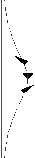
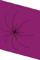
Plotting the tracks of some representative null geodesics through a given event (that is, projecting to the hyperslice $\scriptstyle t \,=\, 0$ ), we obtain a picture which looks suspiciously like the family of all semicircles through a point and orthogonal to the Rindler horizon. (See the figure.)

The Fermat metric

The fact that in the Rindler chart, the projections of null geodesics into any spatial hyperslice for the Rindler observers are simply semicircular arcs can be verified directly from the general solution just given, but there is a very simple way to see this. A static spacetime is one in which a vorticity-free timelike Killing vector field can be found. In this case, we have a uniquely defined family of (identical) spatial hyperslices orthogonal to the corresponding static observers (who need not be inertial observers). This allows us to define a new metric on any of these hyperslices which is conformally related to the original metric inherited from the spacetime, but with the property that geodesics in the new metric (note this is a Riemannian metric on a Riemannian three-manifold) are precisely the projections of the null geodesics of spacetime. This new metric is called the Fermat metric, and in a static spacetime endowed with a coordinate chart in which the line element has the form

ds^2 = g_{00} \, dt^2 + g_{jk} \, dx^j \, dx^k,\;\; j,\; k \in \{1, 2, 3\}

the Fermat metric on $\scriptstyle t \;=\; 0$ is simply

d\rho^2 = \frac{1}{-g_{00}}\left(g_{jk} \, dx^j \, dx^k\right)

(where the metric coeffients are understood to be evaluated at $\scriptstyle t \;=\; 0$ ).

In the Rindler chart, the timelike translation $\scriptstyle \partial_t$ is such a Killing vector field, so this is a static spacetime (not surprisingly, since Minkowski spacetime is of course trivially a static vacuum solution of the Einstein field equation). Therefore, we may immediately write down the Fermat metric for the Rindler observers:

d\rho^2 = \frac{1}{x^2}\left(dx^2 + dy^2 + dz^2\right),\;\; \forall x>0,\;\; \forall y, z

But this is the well-known line element of hyperbolic three-space H³ in the upper half space chart! This is closely analogous to the well known upper half plane chart for the hyperbolic plane H², which is familiar to generations of complex analysis students in connection with conformal mapping problems (and much more), and many mathematically minded readers already know that the geodesics of H² in the upper half plane model are simply semicircles (orthogonal to the circle at infinity represented by the real axis).

Symmetries

Since the Rindler chart is a coordinate chart for Minkowski spacetime, we expect to find ten linearly independent Killing vector fields. Indeed, in the Cartesian chart we can readily find ten linearly independent Killing vector fields, generating respectively one parameter subgroups of time translation, three spatials, three rotations and three boosts. Together these generate the (proper isochronous) Poincaré group, the symmetry group of Minkowski spacetime.

However, it is instructive to write down and solve the Killing vector equations directly. We obtain four familiar looking Killing vector fields

\partial_t, \; \; \partial_y, \; \; \partial_z, \; \; -z \, \partial_y + y \, \partial_z

(time translation, spatial translations orthogonal to the direction of acceleration, and spatial rotation orthogonal to the direction of acceleration) plus six more:

\begin{align} &\exp(\pm t) \, \left( \frac{y}{x} \, \partial_t \pm \left[ y \, \partial_x - x \, \partial_y \right] \right)\\ &\exp(\pm t) \, \left( \frac{z}{x} \, \partial_t \pm \left[ z \, \partial_x - x \, \partial_z \right] \right)\\ &\exp(\pm t) \, \left( \frac{1}{x} \, \partial_t \pm \partial_x \right) \end{align}

(where the signs are chosen consistently + or −). We leave it as an exercise to figure out how these are related to the standard generators; here we wish to point out that we must be able to obtain generators equivalent to $\scriptstyle \partial_T$ in the Cartesian chart, yet the Rindler wedge is obviously not invariant under this translation. How can this be? The answer is that like anything defined by a system of partial differential equations on a smooth manifold, the Killing equation will in general have locally defined solutions, but these might not exist globally. That is, with suitable restrictions on the group parameter, a Killing flow can always be defined in a suitable local neighborhood, but the flow might not be well-defined globally. This has nothing to do with Lorentzian manifolds per se, since the same issue arises in the study of general smooth manifolds.

Notions of distance

One of the many valuable lessons to be learned from a study of the Rindler chart is that there are in fact several distinct (but reasonable) notions of distance which can be used by the Rindler observers.

The first is the one we have tacitly employed above: the induced Riemannian metric on the spatial hyperslices $\scriptstyle t \;=\; t_0$ . We will call this the ruler distance since it corresponds to this induced Riemannian metric, but its operational meaning might not be immediately apparent.

From the standpoint of physical measurement, a more natural notion of distance between two world lines is the radar distance. This is computed by sending a null geodesic from the world line of our observer (event A) to the world line of some small object, whereupon it is reflected (event B) and returns to the observer (event C). The radar distance is then obtained by dividing the round trip travel time, as measured by an ideal clock carried by our observer.

(In Minkowski spacetime, fortunately, we can ignore the possibility of multiple null geodesic paths between two world lines, but in cosmological models and other applications things are not so simple! We should also caution against assuming that this notion of distance between two observers gives a notion which is symmetric under interchanging the observers!)

In particular, let us consider a pair of Rindler observers with coordinates $\scriptstyle x \;=\; x_0, \; y \;=\; 0,\; z \;=\; 0$ and $\scriptstyle x \;=\; x_0 \,+\, h, \; y \;=\; 0,\; \; z \;=\; 0$ respectively. (Note that the first of these, the trailing observer, is accelerating a bit harder, in order to keep up with the leading observer). Setting $\scriptstyle dy \;=\; dz \;=\; 0$ in the Rindler line element, we readily obtain the equation of null geodesics moving in the direction of acceleration:

t-t_{0}=\log \left({\frac {x}{x_{0}}}\right)

Therefore, the radar distance between these two observers is given by

x_0 \, \log \left(1 + \frac{h}{x_0} \right) = h - \frac{h^2}{2 \, x_0} + O \left( h^3 \right)

This is a bit smaller than the ruler distance, but for nearby observers the discrepancy is negligible.

A third possible notion of distance is this: our observer measures the angle subtended by a unit disk placed on some object (not a point object!), as it appears from his location. We call this the optical diameter distance. Because of the simple character of null geodesics in Minkowski spacetime, we can readily determine the optical distance between our pair of Rindler observers (aligned with the direction of acceleration). From a sketch it should be plausible that the optical diameter distance scales like $\scriptstyle h \,+\, \frac{1}{x_0} \,+\, O \left( h^3 \right)$ . Therefore, in the case of a trailing observer estimating distance to a leading observer (the case $\scriptstyle h \,>\, 0$ ), the optical distance is a bit larger than the ruler distance, which is a bit larger than the radar distance. The reader should now take a moment to consider the case of a leading observer estimating distance to a trailing observer!

There are other notions of distance, but the main point is clear: while the values of these various notions will in general disagree for a given pair of Rindler observers, they all agree that every pair of Rindler observers maintains constant distance. The fact that very nearby Rindler observers are mutually stationary follows from the fact, noted above, that the expansion tensor of the Rindler congruence vanishes identically. However, we have shown here that in various senses, this rigidity property holds at larger scales. This is truly a remarkable rigidity property, given the well-known fact that in relativistic physics, no rod can be accelerated rigidly (and no disk can be spun up rigidly) — at least, not without sustaining inhomogeneous stresses. The easiest way to see this is to observe that in Newtonian physics, if we "kick" a rigid body, all elements of matter in the body will immediately change their state of motion. This is of course incompatible with the relativistic principle that no information having any physical effect can be transmitted faster than the speed of light.

It follows that if a rod is accelerated by some external force applied anywhere along its length, the elements of matter in various different places in the rod cannot all feel the same magnitude of acceleration if the rod is not to extend without bound and ultimately break. In other words, an accelerated rod which does not break must sustain stresses which vary along its length. Furthermore, in any thought experiment with time varying forces, whether we "kick" an object or try to accelerate it gradually, we cannot avoid the problem of avoiding mechanical models which are inconsistent with relativistic kinematics (because distant parts of the body respond too quickly to an applied force).

Returning to the question of the operational significance of the ruler distance, we see that this should be the distance which our observers will obtain should they very slowly pass from hand to hand a small ruler which is repeatedly set end to end. But justifying this interpretation in detail would require some kind of material model.

Generalization to curved spacetimes

Rindler coordinates as described above can be generalized to curved spacetime, as Fermi normal coordinates. The generalization essential involves constructing an appropriate orthonormal tetrad and then transporting it along the given trajectory using the Fermi–Walker transport rule. For details, see the paper by Ni and Zimmermann in the references below. Such a generalization actually enables one to study inertial and gravitational effects in an Earth-based laboratory, as well as the more interesting coupled inertial-gravitational effects.

Notes

↑ Einstein, Albert; Rosen, Nathan (1935). "A Particle Problem in the General Theory of Relativity". Physical Review. 48: 73. Bibcode:1935PhRv...48...73E. doi:10.1103/PhysRev.48.73. See equation eqn 1 and footnote 1. They state that this metric is "well known" but provide no reference.
↑ Koks, Don: Explorations in Mathematical Physics (2006), pp. 240-252
↑ Dieter Brill, “Black Hole Horizons and How They Begin”, Astronomical Review (2012); Online Article, cited Sept.2012.

References

Useful background:

Boothby, William M. (1986). An Introduction to Differentiable Manifolds and Riemannian Geometry. New York: Academic Press. ISBN 0-12-116052-1. See Chapter 4 for background concerning vector fields on smooth manifolds.
Frankel, Theodore (1979). Gravitational Curvature: an Introduction to Einstein's Theory. San Francisco : W. H. Freeman. ISBN 0-7167-1062-5. See Chapter 8 for a derivation of the Fermat metric.

Rindler coordinates:

Rindler, Wolfgang (1969). Essential Relativity. New York, Van Nostrand Reinhold Co. doi:10.1007/978-1-4757-1135-6. ISBN 978-0-387-90201-2.

Misner, Charles; Thorne, Kip S. & Wheeler, John Archibald (1973). Gravitation. San Francisco: W. H. Freeman. ISBN 0-7167-0344-0. See Section 6.6.
Rindler, Wolfgang (2001). Relativity: Special, General and Cosmological. Oxford: Oxford University Press. ISBN 0-19-850836-0.
Ni, Wei-Tou; Zimmermann, Mark (1978). "Inertial and gravitational effects in the proper reference frame of an accelerated, rotating observer". Physical Review D. 17 (6): 1473–1476. Bibcode:1978PhRvD..17.1473N. doi:10.1103/PhysRevD.17.1473.

Rindler horizon:

Jacobson, Ted & Parenti, Renaud (2003). "Horizon Entropy". Found. Phys. 33 (2): 323–348. doi:10.1023/A:1023785123428. eprint version
Barceló, Carlos; Liberati, Stefano & Visser, Matt. "Analogue Gravity". Living Reviews in Relativity. Retrieved 2006-05-06.

This article is issued from Wikipedia - version of the 9/8/2016. The text is available under the Creative Commons Attribution/Share Alike but additional terms may apply for the media files.