Range minimum query
In computer science, a range minimum query (RMQ) solves the problem of finding the minimal value in a sub-array of an array of comparable objects. Range minimum queries have several use cases in computer science such as the lowest common ancestor problem or the longest common prefix problem (LCP).
Definition
Given an array A[1 … n] of n objects taken from a well-ordered set (such as numbers), the range minimum query RMQA(l,r) =arg min A[k] (with 1 ≤ l ≤ k ≤ r ≤ n) returns the position of the minimal element in the specified sub-array A[l … r].
For example, when A = [0,5,2,5,4,3,1,6,3], then the answer to the range minimum query for the sub-array A[3 … 8] = [2,5,4,3,1,6] is 7, as A[7] = 1.
Algorithms
Naïve solution
In a typical setting, the array A is static, i.e., elements are not inserted or deleted during a series of queries, and the queries to be answered on-line (i.e., the whole set of queries are not known in advance to the algorithm). In this case a suitable preprocessing of the array into a data structure ensures faster query answering. A naïve solution is to precompute all possible queries, i.e. the minimum of all sub-arrays of A, and store these in an array B such that B[i, j] = min(A[i…j]); then a range min query can be solved in constant time by array lookup in B. There are Θ(n²) possible queries for a length-n array, and the answers to these can be computed in Θ(n²) time by dynamic programming.[1]
Solution using constant time and linearithmic space
As in the solution above, answering queries in constant time will be achieved by pre-computing results. However, the array will store precomputed min queries for all and only the ranges whose size is a power of two. There are Θ(log n) such queries for each start position i, so the size of the dynamic programming table B is Θ(n log n). Each element B[i, j] holds the index of the minimum of the range A[i…i+2j-1]. The table is filled with the indices of minima using the recurrence[1]
- If A[B[i, j-1]] ≤ A[B[i+2j-1, j-1]], then B[i, j] = B[i, j-1];
- else, B[i, j] = B[i+2j-1, j-1].
A query RMQA(l,r) can now be answered by splitting it into two separate queries: one is the pre-computed query with range from l to the highest boundary smaller than r. The other is the query with the same range that has r as its right boundary. The overall result can be obtained in constant time because these two queries can be answered in constant time and the only thing left to do is to choose the smaller of the two results.
| k | |||||
|---|---|---|---|---|---|
| 0 | 1 | 2 | 3 | ||
| l | 1 | 1 | 1 | 1 | 1 |
| 2 | 2 | 3 | 3 | 3 | |
| 3 | 3 | 3 | 3 | 7 | |
| 4 | 4 | 5 | 6 | 7 | |
| 5 | 5 | 6 | 7 | 7 | |
| 6 | 6 | 7 | 7 | 7 | |
| 7 | 7 | 7 | 7 | 7 | |
| 8 | 8 | 7 | 7 | 7 | |
| 9 | 9 | 7 | 7 | 7 | |
Solution using logarithmic time and linear space
This solution answers RMQs in O(log n) time. Its data structures use O(n) space and its data structures can also be used to answer queries in constant time. The array is first conceptually divided into blocks of size s = log n/4. Then the minimum for each block can be computed in O(n) time overall and the minima are stored in a new array.
RMQs can now be answered in logarithmic time by looking at the blocks containing the left query boundary, the right query boundary and all the blocks in between:
- The two blocks containing the boundaries can be searched naïvely. Elements outside the boundary need not even be looked at. This can be done in logarithmic time.
- The minima of all blocks that are fully contained in the range, and the two minima mentioned above, need to be compared to answer the query.
- Because the array was divided into blocks of size log n/4, there are at most 4n/log n blocks that are fully contained in the query.
- By using the linearithmic solution one can find the overall minimum among these blocks. This data structure has size O(n/log n log (n/log n)) = O(n).
- Now, only three minima need to be compared.
For example, using the array A = [0,5,2,5,4,3,1,6,3] and a block size of 3 (for illustrative purposes only) yields the minimum array A' = [0,3,1].
Solution using constant time and linear space
Using the solution above, the sub-queries inside the blocks that are not fully contained in the query still need to be answered in constant time. There are at most two of those blocks: the block containing l and the block containing r. Constant time is achieved by storing the Cartesian trees for all the blocks in the array. A few observations:
- Blocks with isomorphic Cartesian trees give the same result for all queries in that block
- The number of different Cartesian trees of s nodes is Cs, the s'th Catalan number
- Therefore, the number of different Cartesian trees for the blocks is in the range of 4s
For every such tree, the possible result for all queries need to be stored. This comes down to s2 or O(log2 n) entries. This means the overall size of the table is O(n).
To look up results efficiently, the Cartesian tree (row) corresponding to a specific block must be addressable in constant time. The solution is to store the results for all trees in an array and find a unique projection from binary trees to integers to address the entries. This can be achieved by doing a breadth-first-search through the tree and adding leave nodes so that every existing node in the Cartesian tree has exactly two children. The integer is then generated by representing every inner node as a 0-bit and every leaf as a 1-bit in a bit-word (by traversing the tree in level-order again). This leads to a size of log n/4 for every tree. To enable random access in constant time to any tree, the trees not contained in the original array need to be included as well. An array with indices of log n/4 bits length has size 2log n/4 = O(n).

| Index | 1 | 2 | 3 | ||||||
| 1 | 2 | 3 | 1 | 2 | 3 | 1 | 2 | 3 | |
| 0 | / | ||||||||
| 23 (Bitword 0010111) | 1 | 2 | 3 | / | 2 | 3 | / | / | 3 |
| 39 (Bitword 0100111) | 1 | 1 | 1 | / | 2 | 3 | / | / | 3 |
| 127 | / | ||||||||
Applications
RMQs are used as a tool for many tasks in exact and approximate string matching. Several applications can be found in Fischer and Heun (2007).[2]:3
Computing the lowest common ancestor in a tree
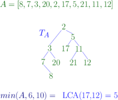
RMQs can be used to solve the lowest common ancestor problem[1][3] and are used as a tool for many tasks in exact and approximate string matching. The LCA query LCAS(v, w) of a rooted tree S = (V, E) and two nodes v, w ∈ V returns the deepest node u (which may be v or w) on paths from the root to both w and v. Gabow, Bentley, and Tarjan (1984) showed that the LCA Problem can be reduced in linear time to the RMQ problem. It follows that, like the RMQ problem, the LCA problem can be solved in constant time and linear space.[2]
Computing the longest common prefix in a string
In the context of text indexing, RMQs can be used to find the LCP (longest common prefix), where LCPT(i, j) computes the LCP of the suffixes that start at indexes i and j in T. To do this we first compute the suffix array A, and the inverse suffix array A−1. We then compute the LCP array H giving the LCP of adjacent suffixes in A. Once these data structures are computed, and RMQ preprocessing is complete, the length of the general LCP can by computed in constant time by the formula: LCP(i, j) = RMQH(A-1[i] + 1, A-1[j]).[4]
See also
References
- Berkman, Omer; Vishkin, Uzi (1993). "Recursive Star-Tree Parallel Data Structure". SIAM Journal on Computing. 22 (2): 221–242. doi:10.1137/0222017.
- 1 2 3 Bender, Michael A.; Farach-Colton, Martín; Pemmasani, Giridhar; Skiena, Steven; Sumazin, Pavel (2005). "Lowest common ancestors in trees and directed acyclic graphs" (PDF). Journal of Algorithms. 57 (2): 75–94. doi:10.1016/j.jalgor.2005.08.001.
- 1 2 Fischer, Johannes; Heun, Volker (2007). A New Succinct Representation of RMQ-Information and Improvements in the Enhanced Suffix Array. Proceedings of the International Symposium on Combinatorics, Algorithms, Probabilistic and Experimental Methodologies. LNCS. 4614. Springer. pp. 459–470. doi:10.1007/978-3-540-74450-4_41.
- ↑ Bender, Michael; Farach-Colton, Martín (2000). The LCA Problem Revisited. LATIN 2000: Theoretical Informatics. LNCS. 1776. Springer. pp. 88–94. doi:10.1007/10719839_9.
- ↑ Fischer, J. and V. Heun (2006). "Theoretical and practical improvements on the RMQ-problem, with applications to LCA and LCE". Combinatorial Pattern Matching: 36–48. doi:10.1007/11780441_5.
External links
- An article on Range Minimum Queries on TopCoder
- Range Minimum Query article on PEGWiki / P3G
- Stanford CS166 RMQ introduction slides