Ramsey–Cass–Koopmans model
The Ramsey–Cass–Koopmans model, or Ramsey growth model, is a neo-classical model of economic growth based primarily on the work of Frank P. Ramsey,[1] with significant extensions by David Cass and Tjalling Koopmans.[2][3] The Ramsey–Cass–Koopmans model differs from the Solow–Swan model in that the choice of consumption is explicitly microfounded at a point in time and so endogenizes the savings rate. As a result, unlike in the Solow–Swan model, the saving rate may not be constant along the transition to the long run steady state. Another implication of the model is that the outcome is Pareto optimal or Pareto efficient.[note 1]
Originally Ramsey set out the model as a central planner's problem of maximizing levels of consumption over successive generations.[4] Only later was a model adopted by Cass and Koopmans as a description of a decentralized dynamic economy. The Ramsey–Cass–Koopmans model aims only at explaining long-run economic growth rather than business cycle fluctuations, and does not include any sources of disturbances like market imperfections, heterogeneity among households, or exogenous shocks. Subsequent researchers therefore extended the model, allowing for government-purchases shocks, variations in employment, and other sources of disturbances, which is known as real business cycle theory.
Key equations
Like the Solow–Swan model, the Ramsey–Cass–Koopmans model starts with an aggregate production function that satisfies the Inada conditions, of Cobb–Douglas type, , with factors capital , labour , and labour-augmenting technology . The amount of labour is equal to the population in the economy, and grows at a constant rate . Likewise, the level of technology grows at a constant rate . The first key equation of the Ramsey–Cass–Koopmans model is the law of motion for capital accumulation:


where is capital intensity (capital per worker), is change in capital per worker over time (), is consumption per worker, is output per worker, and is the depreciation rate of capital. Under the simplifying assumption that there is neither population growth nor an increase in technology level, this equation states that investment, or increase in capital per worker is that part of output which is not consumed, minus the rate of depreciation of capital. Investment is, therefore, the same as savings.


It also yields a potentially optimal steady-state of the growth model, in which , i.e. no (further) change in capital intensity. Now, one has to determine the steady-state which maximizes consumption , and yields an optimal savings rate . This is the "golden rule" optimality condition proposed by Edmund Phelps in 1961.[5]


where is the level of investment, is level of income and is the savings rate, or the proportion of income that is saved.


The second equation concerns the saving behavior of households and is less intuitive. If households are maximizing their consumption intertemporally, at each point in time they equate the marginal benefit of consumption today with that of consumption in the future, or equivalently, the marginal benefit of consumption in the future with its marginal cost. Because this is an intertemporal problem this means an equalization of rates rather than levels. There are two reasons why households prefer to consume now rather than in the future. First, they discount future consumption. Second, because the utility function is concave, households prefer a smooth consumption path. An increasing or a decreasing consumption path lowers the utility of consumption in the future. Hence the following relationship characterizes the optimal relationship between the various rates:
rate of return on savings = rate at which consumption is discounted − percent change in marginal utility times the growth of consumption.
Mathematically:

A class of utility functions which are consistent with a steady state of this model are the isoelastic or constant relative risk aversion (CRRA) utility functions, given by:

In this case we have:

Then solving the above dynamic equation for consumption growth we get:

which is the second key dynamic equation of the model and is usually called the "Euler equation".
With a neoclassical production function with constant returns to scale, the interest rate, r, will equal the marginal product of capital per worker. One particular case is given by the Cobb–Douglas production function

which implies that the gross interest rate is

hence the net interest rate r

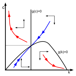
Setting and equal to zero we can find the steady state of this model.

History
Spear and Young re-examine the history of optimal growth during the 1950s and 1960s,[6] focusing in part on the veracity of the claimed simultaneous and independent development of Cass' "Optimum growth in an aggregative model of capital accumulation" (published in 1965 in the Review of Economic Studies), and Tjalling Koopman's "On the concept of optimal economic growth" (published in Study Week on the Econometric Approach to Development Planning, 1965, Rome: Pontifical Academy of Science).
Over their lifetimes, neither Cass nor Koopmans ever suggested that their results characterizing optimal growth in the one-sector, continuous-time growth model were anything other than "simultaneous and independent". That the issue of priority ever became a discussion point was due only to the fact that in the published version of Koopmans' work, he cited the chapter from Cass' thesis that later became the RES paper. In his paper, Koopmans states in a footnote that Cass independently obtained conditions similar to what Koopmans finds, and that Cass also considers the limiting case where the discount rate goes to zero in his paper. For his part, Cass notes that "after the original version of this paper was completed, a very similar analysis by Koopmans came to our attention. We draw on his results in discussing the limiting case, where the effective social discount rate goes to zero". In the interview that Cass gave to Macroeconomic Dynamics, he credits Koopmans with pointing him to Frank Ramsey's previous work, claiming to have been embarrassed not to have known of it, but says nothing to dispel the basic claim that his work and Koopmans' were in fact independent.
Spear and Young dispute this history, based upon a previously overlooked working paper version of Koopmans' paper,[7] which was the basis for Koopmans' oft-cited presentation at a conference held by the Pontifical Academy of Sciences in October 1963.[8] In this Cowles Discussion paper, there is an error. Koopmans claims in his main result that the Euler equations are both necessary and sufficient to characterize optimal trajectories in the model because any solutions to the Euler equations which do not converge to the optimal steady-state would hit either a zero consumption or zero capital boundary in finite time. This error was apparently presented at the Vatican conference, although at the time of Koopmans' presenting it, no participant commented on the problem. This can be inferred because the discussion after each paper presentation at the Vatican conference is preserved verbatim in the conference volume.
In the Vatican volume discussion following the presentation of a paper by Edmond Malinvaud, the issue does arise because of Malinvaud's explicit inclusion of a so-called "transversality condition" (which Malinvaud calls Condition I) in his paper. At the end of the presentation, Koopmans asks Malinvaud whether it is not the case that Condition I simply guarantees that solutions to the Euler equations that do not converge to the optimal steady-state hit a boundary in finite time. Malinvaud replies that this is not the case, and suggests that Koopmans look at the example with log utility functions and Cobb-Douglas production functions.
At this point, Koopmans obviously recognizes he has a problem, but, based on a confusing appendix to a later version of the paper produced after the Vatican conference, he seems unable to decide how to deal with the issue raised by Malinvaud's Condition I.
From the Macroeconomic Dynamics interview with Cass, it is clear that Koopmans met with Cass' thesis advisor, Hirofumi Uzawa, at the winter meetings of the Econometric Society in January 1964, where Uzawa advised him that his student [Cass] had solved this problem already. Uzawa must have then provided Koopmans with the copy of Cass' thesis chapter, which he apparently sent along in the guise of the IMSSS Technical Report that Koopmans cited in the published version of his paper. The word "guise" is appropriate here, because the TR number listed in Koopmans' citation would have put the issue date of the report in the early 1950s, which it clearly was not.
In the published version of Koopmans' paper, he imposes a new Condition Alpha in addition to the Euler equations, stating that the only admissible trajectories among those satisfying the Euler equations is the one that converges to the optimal steady-state equilibrium of the model. This result is derived in Cass' paper via the imposition of a transversality condition that Cass deduced from relevant sections of a book by Lev Pontryagin, Vladimir Boltyansky, Revaz Gamkrelidze, and Evgenii Mishchenko.[9] Spear and Young conjecture that Koopmans took this route because he did not want to appear to be "borrowing" either Malinvaud's or Cass' transversality technology.
Based on this and other examination of Malinvaud's contributions in 1950s—specifically his intuition of the importance of the transversality condition—Spear and Young suggest that the neo-classical growth model might better be called the Ramsey–Malinvaud–Cass model than the established Ramsey–Cass–Koopmans honorific.
Notes
- ↑ This result is due not just to the endogeneity of the saving rate but also because of the infinite nature of the planning horizon of the agents in the model; it does not hold in other models with endogenous saving rates but more complex intergenerational dynamics, for example, in Samuelson's or Diamond's overlapping generations models.
References
- ↑ Ramsey, Frank P. (1928). "A Mathematical Theory of Saving". Economic Journal. 38 (152): 543–559. JSTOR 2224098.
- ↑ Cass, David (1965). "Optimum Growth in an Aggregative Model of Capital Accumulation". Review of Economic Studies. 32 (3): 233–240. JSTOR 2295827.
- ↑ Koopmans, T. C. (1965). "On the Concept of Optimal Economic Growth". The Economic Approach to Development Planning. Chicago: Rand McNally. pp. 225–287.
- ↑ Collard, David A. (2011). "Ramsey, saving and the generations". Generations of Economists. London: Routledge. pp. 256–273. ISBN 978-0-415-56541-7.
- ↑ Phelps, Edmund (1961). "The Golden Rule of Accumulation: A Fable for Growthmen". American Economic Review. 51 (4): 638–643. JSTOR 1812790.
- ↑ Spear, S. E.; Young, W. (2014). "Optimum Savings and Optimal Growth: The Cass–Malinvaud–Koopmans Nexus". Macroeconomic Dynamics. 18 (1): 215–243. doi:10.1017/S1365100513000291.
- ↑ Koopmans, Tjalling (December 1963). "On the Concept of Optimal Economic Growth" (PDF). Cowles Foundation Discussion paper 163.
- ↑ McKenzie, Lionel (2002). "Some Early Conferences on Growth Theory". In Bitros, George; Katsoulacos, Yannis. Essays in Economic Theory, Growth and Labor Markets. Cheltenham: Edward Elgar. pp. 3–18. ISBN 1-84064-739-6.
- ↑ Pontryagin, Lev; Boltyansky, Vladimir; Gamkrelidze, Revaz; Mishchenko, Evgenii (1962). The Mathematical Theory of Optimal Processes. New York: John Wiley.
Further reading
- Acemoğlu, Daron (2009). "The Neoclassical Growth Model". Introduction to Modern Economic Growth. Princeton: Princeton University Press. pp. 287–326. ISBN 978-0-691-13292-1.
- Barro, Robert J.; Sala-i-Martin, Xavier (2004). "Growth Models with Consumer Optimization". Economic Growth (Second ed.). New York: McGraw-Hill. pp. 85–142. ISBN 0-262-02553-1.
- Bénassy, Jean-Pascal (2011). "The Ramsey Model". Macroeconomic Theory. New York: Oxford University Press. pp. 145–160. ISBN 978-0-19-538771-1.
- Blanchard, Olivier Jean; Fischer, Stanley (1989). "Consumption and Investment: Basic Infinite Horizon Models". Lectures on Macroeconomics. Cambridge: MIT Press. pp. 37–89. ISBN 0-262-02283-4.
- Miao, Jianjun (2014). "Neoclassical Growth Models". Economic Dynamics in Discrete Time. Cambridge: MIT Press. pp. 353–364. ISBN 978-0-262-02761-8.
- Novales, Alfonso; Fernández, Esther; Ruíz, Jesús (2009). "Optimal Growth: Continuous Time Analysis". Economic Growth: Theory and Numerical Solution Methods. Berlin: Springer. pp. 101–154. ISBN 978-3-540-68665-1.
- Romer, David (2011). "Infinite-Horizon and Overlapping-Generations Models". Advanced Macroeconomics (Fourth ed.). New York: McGraw-Hill. pp. 49–77. ISBN 978-0-07-351137-5.