Program evaluation and review technique

For other uses, see Pert (disambiguation).

PERT network chart for a seven-month project with five milestones (10 through 50) and six activities (A through F).

The program (or project) evaluation and review technique, commonly abbreviated PERT, is a statistical tool, used in project management, which was designed to analyze and represent the tasks involved in completing a given project. First developed by the United States Navy in the 1950s, it is commonly used in conjunction with the critical path method (CPM).

History

Program evaluation and review technique

     The Navy's Special Projects Office, charged with developing the Polaris-Submarine weapon system and the Fleet Ballistic Missile capability, has developed a statistical technique for measuring and forecasting progress in research and development programs. This program evaluation and review technique (code-named PERT) is applied as a decision-making tool designed to save time in achieving end-objectives, and is of particular interest to those engaged in research and development programs for which time is a critical factor.
     The new technique takes recognition of three factors that influence successful achievement of research and development program objectives: time, resources, and technical performance specifications. PERT employs time as the variable that reflects planned resource-applications and performance specifications. With units of time as a common denominator, PERT quantifies knowledge about the uncertainties involved in developmental programs requiring effort at the edge of, or beyond, current knowledge of the subject — effort for which little or no previous experience exists.
     Through an electronic computer, the PERT technique processes data representing the major, finite accomplishments (events) essential to achieve end-objectives; the inter-dependence of those events; and estimates of time and range of time necessary to complete each activity between two successive events. Such time expectations include estimates of "most likely time", "optimistic time", and "pessimistic time" for each activity. The technique is a management control tool that sizes up the outlook for meeting objectives on time; highlights danger signals requiring management decisions; reveals and defines both methodicalness and slack in the flow plan or the network of sequential activities that must be performed to meet objectives; compares current expectations with scheduled completion dates and computes the probability for meeting scheduled dates; and simulates the effects of options for decision — before decision.

     The concept of PERT was developed by an operations research team staffed with representatives from the Operations Research Department of Booz, Allen and Hamilton; the Evaluation Office of the Lockheed Missile Systems Division; and the Program Evaluation Branch, Special Projects Office, of the Department of the Navy.
— Willard Fazar (Head, Program Evaluation Branch, Special Projects Office, U.S. Navy), The American Statistician, April 1959.^[1]

Overview

PERT is a method to analyze the involved tasks in completing a given project, especially the time needed to complete each task, and to identify the minimum time needed to complete the total project.

PERT was developed primarily to simplify the planning and scheduling of large and complex projects. It was developed for the U.S. Navy Special Projects Office in 1957 to support the U.S. Navy's Polaris nuclear submarine project.^[2] It was able to incorporate uncertainty by making it possible to schedule a project while not knowing precisely the details and durations of all the activities. It is more of an event-oriented technique rather than start- and completion-oriented, and is used more in projects where time is the major factor rather than cost. It is applied to very large-scale, one-time, complex, non-routine infrastructure and Research and Development projects. An example of this was for the 1968 Winter Olympics in Grenoble which applied PERT from 1965 until the opening of the 1968 Games.^[3]

This project model was the first of its kind, a revival for scientific management, founded by Frederick Taylor (Taylorism) and later refined by Henry Ford (Fordism). DuPont's critical path method was invented at roughly the same time as PERT.

Terminology

PERT event: a point that marks the start or completion of one or more activities. It consumes no time and uses no resources. When it marks the completion of one or more activities, it is not "reached" (does not occur) until all of the activities leading to that event have been completed.
predecessor event: an event that immediately precedes some other event without any other events intervening. An event can have multiple predecessor events and can be the predecessor of multiple events.
successor event: an event that immediately follows some other event without any other intervening events. An event can have multiple successor events and can be the successor of multiple events.
PERT activity: the actual performance of a task which consumes time and requires resources (such as labor, materials, space, machinery). It can be understood as representing the time, effort, and resources required to move from one event to another. A PERT activity cannot be performed until the predecessor event has occurred.
PERT sub-activity: a PERT activity can be further decomposed into a set of sub-activities. For example, activity A1 can be decomposed into A1.1, A1.2 and A1.3. Sub-activities have all the properties of activities; in particular, a sub-activity has predecessor or successor events just like an activity. A sub-activity can be decomposed again into finer-grained sub-activities.
optimistic time: the minimum possible time required to accomplish an activity (o) or a path (O), assuming everything proceeds better than is normally expected
pessimistic time: the maximum possible time required to accomplish an activity (p) or a path (P), assuming everything goes wrong (but excluding major catastrophes).
most likely time: the best estimate of the time required to accomplish an activity (m) or a path (M), assuming everything proceeds as normal.
expected time: the best estimate of the time required to accomplish an activity (te) or a path (TE), accounting for the fact that things don't always proceed as normal (the implication being that the expected time is the average time the task would require if the task were repeated on a number of occasions over an extended period of time).

te = (o + 4m + p) ÷ 6

TE=\sum _{i=1}^{n}te_{i}

standard deviation of time : the variability of the time for accomplishing an activity (σ_te) or a path (σ_TE)

σ_te = (p - o) ÷ 6

\sigma _{TE}={\sqrt {\sum _{i=1}^{n}{\sigma _{te_{i}}}^{2}}}

float or slack is a measure of the excess time and resources available to complete a task. It is the amount of time that a project task can be delayed without causing a delay in any subsequent tasks (free float) or the whole project (total float). Positive slack would indicate ahead of schedule; negative slack would indicate behind schedule; and zero slack would indicate on schedule.
critical path: the longest possible continuous pathway taken from the initial event to the terminal event. It determines the total calendar time required for the project; and, therefore, any time delays along the critical path will delay the reaching of the terminal event by at least the same amount.
critical activity: An activity that has total float equal to zero. An activity with zero float is not necessarily on the critical path since its path may not be the longest.
Lead time: the time by which a predecessor event must be completed in order to allow sufficient time for the activities that must elapse before a specific PERT event reaches completion.
lag time: the earliest time by which a successor event can follow a specific PERT event.
fast tracking: performing more critical activities in parallel
crashing critical path: Shortening duration of critical activities

Implementation

The first step to scheduling the project is to determine the tasks that the project requires and the order in which they must be completed. The order may be easy to record for some tasks (e.g. When building a house, the land must be graded before the foundation can be laid) while difficult for others (There are two areas that need to be graded, but there are only enough bulldozers to do one). Additionally, the time estimates usually reflect the normal, non-rushed time. Many times, the time required to execute the task can be reduced for an additional cost or a reduction in the quality.

In the following example there are seven tasks, labeled A through G. Some tasks can be done concurrently (A and B) while others cannot be done until their predecessor task is complete (C cannot begin until A is complete). Additionally, each task has three time estimates: the optimistic time estimate (o), the most likely or normal time estimate (m), and the pessimistic time estimate (p). The expected time (te) is computed using the formula (o + 4m + p) ÷ 6.

Activity	Predecessor	Time estimates			Expected time
Activity	Predecessor	Opt. (o)	Normal (m)	Pess. (p)	Expected time
A	—	2	4	6	4.00
B	—	3	5	9	5.33
C	A	4	5	7	5.17
D	A	4	6	10	6.33
E	B, C	4	5	7	5.17
F	D	3	4	8	4.50
G	E	3	5	8	5.17

Once this step is complete, one can draw a Gantt chart or a network diagram.

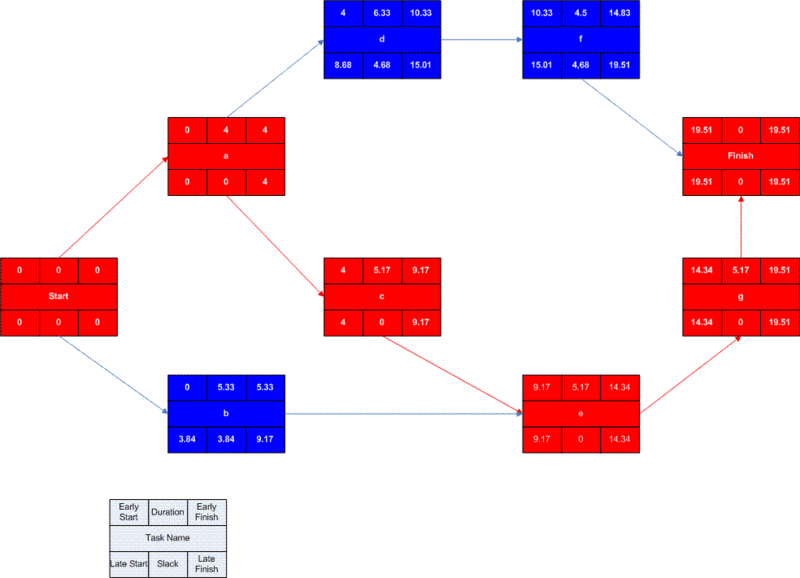
A network diagram can be created by hand or by using diagram software. There are two types of network diagrams, activity on arrow (AOA) and activity on node (AON). Activity on node diagrams are generally easier to create and interpret. To create an AON diagram, it is recommended (but not required) to start with a node named start. This "activity" has a duration of zero (0). Then you draw each activity that does not have a predecessor activity (a and b in this example) and connect them with an arrow from start to each node. Next, since both c and d list a as a predecessor activity, their nodes are drawn with arrows coming from a. Activity e is listed with b and c as predecessor activities, so node e is drawn with arrows coming from both b and c, signifying that e cannot begin until both b and c have been completed. Activity f has d as a predecessor activity, so an arrow is drawn connecting the activities. Likewise, an arrow is drawn from e to g. Since there are no activities that come after f or g, it is recommended (but again not required) to connect them to a node labeled finish.

By itself, the network diagram pictured above does not give much more information than a Gantt chart; however, it can be expanded to display more information. The most common information shown is:

The activity name
The normal duration time
The early start time (ES)
The early finish time (EF)
The late start time (LS)
The late finish time (LF)
The slack

In order to determine this information it is assumed that the activities and normal duration times are given. The first step is to determine the ES and EF. The ES is defined as the maximum EF of all predecessor activities, unless the activity in question is the first activity, for which the ES is zero (0). The EF is the ES plus the task duration (EF = ES + duration).

The ES for start is zero since it is the first activity. Since the duration is zero, the EF is also zero. This EF is used as the ES for a and b.
The ES for a is zero. The duration (4 work days) is added to the ES to get an EF of four. This EF is used as the ES for c and d.
The ES for b is zero. The duration (5.33 work days) is added to the ES to get an EF of 5.33.
The ES for c is four. The duration (5.17 work days) is added to the ES to get an EF of 9.17.
The ES for d is four. The duration (6.33 work days) is added to the ES to get an EF of 10.33. This EF is used as the ES for f.
The ES for e is the greatest EF of its predecessor activities (b and c). Since b has an EF of 5.33 and c has an EF of 9.17, the ES of e is 9.17. The duration (5.17 work days) is added to the ES to get an EF of 14.34. This EF is used as the ES for g.
The ES for f is 10.33. The duration (4.5 work days) is added to the ES to get an EF of 14.83.
The ES for g is 14.34. The duration (5.17 work days) is added to the ES to get an EF of 19.51.
The ES for finish is the greatest EF of its predecessor activities (f and g). Since f has an EF of 14.83 and g has an EF of 19.51, the ES of finish is 19.51. Finish is a milestone (and therefore has a duration of zero), so the EF is also 19.51.

Barring any unforeseen events, the project should take 19.51 work days to complete. The next step is to determine the late start (LS) and late finish (LF) of each activity. This will eventually show if there are activities that have slack. The LF is defined as the minimum LS of all successor activities, unless the activity is the last activity, for which the LF equals the EF. The LS is the LF minus the task duration (LS = LF − duration).

The LF for finish is equal to the EF (19.51 work days) since it is the last activity in the project. Since the duration is zero, the LS is also 19.51 work days. This will be used as the LF for f and g.
The LF for g is 19.51 work days. The duration (5.17 work days) is subtracted from the LF to get an LS of 14.34 work days. This will be used as the LF for e.
The LF for f is 19.51 work days. The duration (4.5 work days) is subtracted from the LF to get an LS of 15.01 work days. This will be used as the LF for d.
The LF for e is 14.34 work days. The duration (5.17 work days) is subtracted from the LF to get an LS of 9.17 work days. This will be used as the LF for b and c.
The LF for d is 15.01 work days. The duration (6.33 work days) is subtracted from the LF to get an LS of 8.68 work days.
The LF for c is 9.17 work days. The duration (5.17 work days) is subtracted from the LF to get an LS of 4 work days.
The LF for b is 9.17 work days. The duration (5.33 work days) is subtracted from the LF to get an LS of 3.84 work days.
The LF for a is the minimum LS of its successor activities. Since c has an LS of 4 work days and d has an LS of 8.68 work days, the LF for a is 4 work days. The duration (4 work days) is subtracted from the LF to get an LS of 0 work days.
The LF for start is the minimum LS of its successor activities. Since a has an LS of 0 work days and b has an LS of 3.84 work days, the LS is 0 work days.

The next step is to determine the critical path and if any activities have slack. The critical path is the path that takes the longest to complete. To determine the path times, add the task durations for all available paths. Activities that have slack can be delayed without changing the overall time of the project. Slack is computed in one of two ways, slack = LF − EF or slack = LS − ES. Activities that are on the critical path have a slack of zero (0).

The duration of path adf is 14.83 work days.
The duration of path aceg is 19.51 work days.
The duration of path beg is 15.67 work days.

The critical path is aceg and the critical time is 19.51 work days. It is important to note that there can be more than one critical path (in a project more complex than this example) or that the critical path can change. For example, let's say that activities d and f take their pessimistic (b) times to complete instead of their expected (T_E) times. The critical path is now adf and the critical time is 22 work days. On the other hand, if activity c can be reduced to one work day, the path time for aceg is reduced to 15.34 work days, which is slightly less than the time of the new critical path, beg (15.67 work days).

Assuming these scenarios do not happen, the slack for each activity can now be determined.

Start and finish are milestones and by definition have no duration, therefore they can have no slack (0 work days).
The activities on the critical path by definition have a slack of zero; however, it is always a good idea to check the math anyway when drawing by hand.
- LF_a – EF_a = 4 − 4 = 0
- LF_c – EF_c = 9.17 − 9.17 = 0
- LF_e – EF_e = 14.34 − 14.34 = 0
- LF_g – EF_g = 19.51 − 19.51 = 0
Activity b has an LF of 9.17 and an EF of 5.33, so the slack is 3.84 work days.
Activity d has an LF of 15.01 and an EF of 10.33, so the slack is 4.68 work days.
Activity f has an LF of 19.51 and an EF of 14.83, so the slack is 4.68 work days.

Therefore, activity b can be delayed almost 4 work days without delaying the project. Likewise, activity d or activity f can be delayed 4.68 work days without delaying the project (alternatively, d and f can be delayed 2.34 work days each).

A completed network diagram created using Microsoft Visio. Note the critical path is in red.

Advantages

PERT chart explicitly defines and makes visible dependencies (precedence relationships) between the work breakdown structure (commonly WBS) elements.
PERT facilitates identification of the critical path and makes this visible.
PERT facilitates identification of early start, late start, and slack for each activity.
PERT provides for potentially reduced project duration due to better understanding of dependencies leading to improved overlapping of activities and tasks where feasible.
The large amount of project data can be organized and presented in diagram for use in decision making.
PERT can provide a probability of completing before a given time.

Disadvantages

There can be potentially hundreds or thousands of activities and individual dependency relationships.
PERT is not easily scalable for smaller projects.
The network charts tend to be large and unwieldy requiring several pages to print and requiring specially sized paper.
The lack of a timeframe on most PERT/CPM charts makes it harder to show status although colours can help (e.g., specific colour for completed nodes).

Uncertainty in project scheduling

During project execution, however, a real-life project will never execute exactly as it was planned due to uncertainty. This can be due to ambiguity resulting from subjective estimates that are prone to human errors or can be the result of variability arising from unexpected events or risks. The main reason that PERT may provide inaccurate information about the project completion time is due to this schedule uncertainty. This inaccuracy may be large enough to render such estimates as not helpful.

One possible method to maximize solution robustness is to include safety in the baseline schedule in order to absorb the anticipated disruptions. This is called proactive scheduling. A pure proactive scheduling is a utopia; incorporating safety in a baseline schedule which allows for every possible disruption would lead to a baseline schedule with a very large make-span. A second approach, termed reactive scheduling, consists of defining a procedure to react to disruptions that cannot be absorbed by the baseline schedule.

References

↑ B. Ralph Stauber, H. M. Douty, Willard Fazar, Richard H. Jordan, William Weinfeld and Allen D. Manvel. Federal Statistical Activities. The American Statistician 13(2): 9-12 (Apr., 1959) , pp. 9-12
↑ Malcolm, D. G., J. H. Roseboom, C. E. Clark, W. Fazar Application of a Technique for Research and Development Program Evaluation OPERATIONS RESEARCH Vol. 7, No. 5, September–October 1959, pp. 646–669
↑ 1968 Winter Olympics official report. p. 49. Accessed 1 November 2010. (English) & (French)