Power transform
In statistics, a power transform is a family of functions that are applied to create a monotonic transformation of data using power functions. This is a useful data transformation technique used to stabilize variance, make the data more normal distribution-like, improve the validity of measures of association such as the Pearson correlation between variables and for other data stabilization procedures.
Definition
The power transformation is defined as a continuously varying function, with respect to the power parameter λ, in a piece-wise function form that makes it continuous at the point of singularity (λ = 0). For data vectors (y1,..., yn) in which each yi > 0, the power transform is
![y_{i}^{(\lambda )}={\begin{cases}{\dfrac {y_{i}^{\lambda }-1}{\lambda (\operatorname {GM} (y))^{\lambda -1}}},&{\text{if }}\lambda \neq 0\\[12pt]\operatorname {GM} (y)\ln {y_{i}},&{\text{if }}\lambda =0\end{cases}}](../I/m/8c74fb82826bbd941780fe964a283aef93c84f44.svg)
where

is the geometric mean of the observations y1, ..., yn. The case for is the limit as approaches 0. To see this, note that = = . Then = , and everything but becomes negligible for sufficiently small.


The inclusion of the (λ − 1)th power of the geometric mean in the denominator simplifies the scientific interpretation of any equation involving , because the units of measurement do not change as λ changes.

Box and Cox (1964) introduced the geometric mean into this transformation by first including the Jacobian of rescaled power transformation
- .

with the likelihood. This Jacobian is as follows:

This allows the normal log likelihood at its maximum to be written as follows:


From here, absorbing into the expression for produces an expression that establishes that minimizing the sum of squares of residuals from is equivalent to maximizing the sum of the normal log likelihood of deviations from and the log of the Jacobian of the transformation.


The value at Y = 1 for any λ is 0, and the derivative with respect to Y there is 1 for any λ. Sometimes Y is a version of some other variable scaled to give Y = 1 at some sort of average value.
The transformation is a power transformation, but done in such a way as to make it continuous with the parameter λ at λ = 0. It has proved popular in regression analysis, including econometrics.
Box and Cox also proposed a more general form of the transformation that incorporates a shift parameter.

which holds if yi + α > 0 for all i. If τ(Y, λ, α) follows a truncated normal distribution, then Y is said to follow a Box–Cox distribution.
Bickel and Doksum eliminated the need to use a truncated distribution by extending the range of the transformation to all y, as follows:
- ,

where sgn(.) is the Sign function. This change in definition has little practical import as long as is less than , which it usually is.[1]


Bickel and Doksum also proved that the parameter estimates are consistent and asymptotically normal under appropriate regularity conditions, though the standard Cramér–Rao lower bound can substantially underestimate the variance when parameter values are small relative to the noise variance.[1] However, this problem of underestimating the variance may not be a substantive problem in many applications.[2][3]
Box–Cox transformation
The one-parameter Box–Cox transformations are defined as:
![y_{i}^{(\lambda )}={\begin{cases}{\dfrac {y_{i}^{\lambda }-1}{\lambda }}&{\text{if }}\lambda \neq 0,\\[8pt]\ln {(y_{i})}&{\text{if }}\lambda =0,\end{cases}}](../I/m/f82193f340d8158f065346075137bafc270e3401.svg)
and the two-parameter Box-Cox transformations as:
![y_{i}^{({\boldsymbol {\lambda }})}={\begin{cases}{\dfrac {(y_{i}+\lambda _{2})^{\lambda _{1}}-1}{\lambda _{1}}}&{\text{if }}\lambda _{1}\neq 0,\\[8pt]\ln {(y_{i}+\lambda _{2})}&{\text{if }}\lambda _{1}=0,\end{cases}}](../I/m/79b7e533916d38c503eebd45a7fb28ec758b7287.svg)
as described in the original article.[4][5] Moreover, the first transformations hold for and the second for .[4]


The parameter is estimated using the profile likelihood function.
Confidence interval
Confidence interval for the Box-Cox transformation can be asymptotically constructed using Wilks's theorem on the profile likelihood function to find all the possible values of that fulfill the following restriction:[6]

Use of the power transform
- Power transforms are ubiquitously used in various fields. For example, multi-resolution and wavelet analysis, statistical data analysis, medical research, modeling of physical processes, geochemical data analysis, epidemiology[7] and many other clinical, environmental and social research areas.
Example
The BUPA liver data set[8] contains data on liver enzymes ALT and γGT. Suppose we are interested in using log(γGT) to predict ALT. A plot of the data appears in panel (a) of the figure. There appears to be non-constant variance, and a Box–Cox transformation might help.
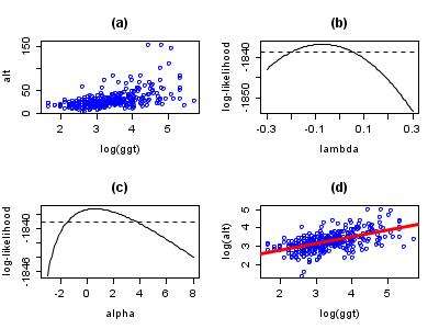
The log-likelihood of the power parameter appears in panel (b). The horizontal reference line is at a distance of χ12/2 from the maximum and can be used to read off an approximate 95% confidence interval for λ. It appears as though a value close to zero would be good, so we take logs.
Possibly, the transformation could be improved by adding a shift parameter to the log transformation. Panel (c) of the figure shows the log-likelihood. In this case, the maximum of the likelihood is close to zero suggesting that a shift parameter is not needed. The final panel shows the transformed data with a superimposed regression line.
Note that although Box–Cox transformations can make big improvements in model fit, there are some issues that the transformation cannot help with. In the current example, the data are rather heavy-tailed so that the assumption of normality is not realistic and a robust regression approach leads to a more precise model.
Econometric application
Economists often characterize production relationships by some variant of the Box–Cox transformation.
Consider a common representation of production Q as dependent on services provided by a capital stock K and by labor hours N:

Solving for Q by inverting the Box–Cox transformation we find

which is known as the constant elasticity of substitution (CES) production function.
The CES production function is a homogeneous function of degree one.
When λ = 1, this produces the linear production function:

When λ → 0 this produces the famous Cobb–Douglas production function:

Activities and demonstrations
The SOCR resource pages contain a number of hands-on interactive activities[9] demonstrating the Box–Cox (Power) Transformation using Java applets and charts. These directly illustrate the effects of this transform on Q-Q plots, X-Y scatterplots, time-series plots and histograms.
Notes
- 1 2 Bickel, Peter J.; Doksum, Kjell A. (June 1981). "An analysis of transformations revisited". Journal of the American Statistical Association. American Statistical Association. 76 (374): 296–311. doi:10.1080/01621459.1981.10477649.
- ↑ Sakia, R. M. (1992), "The Box-Cox transformation technique: a review", The Statistician, 41: 169–178, doi:10.2307/2348250
- ↑ Li, Fengfei (April 11, 2005), Box-Cox Transformations: An Overview (PDF) (slide presentation), Sao Paulo, Brazil: University of Sao Paulo, Brazil, retrieved 2014-11-02
- 1 2 Box, George E. P.; Cox, D. R. (1964). "An analysis of transformations". Journal of the Royal Statistical Society, Series B. 26 (2): 211–252. JSTOR 2984418. MR 192611.
- ↑ Johnston, J. (1984). Econometric Methods (Third ed.). New York: McGraw-Hill. pp. 61–74. ISBN 0-07-032685-1.
- ↑ Abramovich, Felix, and Ya'acov Ritov. Statistical Theory: A Concise Introduction. CRC Press, 2013. Pages 121-122
- ↑ Peters, J. L.; Rushton, L.; Sutton, A. J.; Jones, D. R.; Abrams, K. R.; Mugglestone, M. A. (2005). "Bayesian methods for the cross-design synthesis of epidemiological and toxicological evidence". Journal of the Royal Statistical Society: Series C (Applied Statistics). 54: 159. doi:10.1111/j.1467-9876.2005.00476.x.
- ↑ BUPA liver disorder dataset
- ↑ Power Transform Family Graphs, SOCR webpages
References
- Box, George E. P.; Cox, D. R. (1964). "An analysis of transformations". Journal of the Royal Statistical Society, Series B. 26 (2): 211–252. JSTOR 2984418. MR 192611.
- Carroll, RJ and Ruppert, D. On prediction and the power transformation family. Biometrika 68: 609–615.
- DeGroot, M. H. (1987). "A Conversation with George Box". Statistical Science. 2 (3): 239–258. doi:10.1214/ss/1177013223.
- Handelsman, DJ. Optimal Power Transformations for Analysis of Sperm Concentration and Other Semen Variables. Journal of Andrology, Vol. 23, No. 5, September/October 2002.
- Gluzman, S.; Yukalov, V. I. (2006). "Self-similar power transforms in extrapolation problems". Journal of Mathematical Chemistry. 39 (1): 47–56. doi:10.1007/s10910-005-9003-7.
- Howarth, R. J.; Earle, S. A. M. (1979). "Application of a generalized power transformation to geochemical data". Journal Mathematical Geology. 11 (1): 45–62. doi:10.1007/BF01043245.
External links
- Nishii, R. (2001), "Box–Cox transformation", in Hazewinkel, Michiel, Encyclopedia of Mathematics, Springer, ISBN 978-1-55608-010-4 (fixed link)