Spherical trigonometry

"Spherical triangle" redirects here. For triangles in the Euclidean plane with circular-arc sides, see Reuleaux triangle.

Spherical trigonometry is the branch of spherical geometry that deals with the relationships between trigonometric functions of the sides and angles of the spherical polygons (especially spherical triangles) defined by a number of intersecting great circles on the sphere. Spherical trigonometry is of great importance for calculations in astronomy, geodesy and navigation.

The origins of spherical trigonometry in Greek mathematics and the major developments in Islamic mathematics are discussed fully in History of trigonometry and Mathematics in medieval Islam. The subject came to fruition in Early Modern times with important developments by John Napier, Delambre and others, and attained an essentially complete form by the end of the nineteenth century with the publication of Todhunter's textbook Spherical trigonometry for the use of colleges and Schools. This book is now readily available on the web.^[1] The only significant developments since then have been the application of vector methods for the derivation of the theorems and the use of computers to carry through lengthy calculations.

Preliminaries

Eight spherical triangles defined by the intersection of three great circles.

Spherical polygons

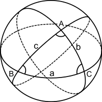
A spherical polygon on the surface of the sphere is defined by a number of great circle arcs that are the intersection of the surface with planes through the centre of the sphere. Such polygons may have any number of sides. Two planes define a lune, also called a "digon" or bi-angle, the two-sided analogue of the triangle: a familiar example is the curved surface of a segment of an orange. Three planes define a spherical triangle, the principal subject of this article. Four planes define a spherical quadrilateral: such a figure, and higher sided polygons, can always be treated as a number of spherical triangles.

From this point the article will be restricted to spherical triangles, denoted simply as triangles.

Notation

The basic triangle on a unit sphere.

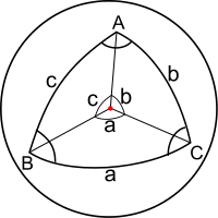
Both vertices and angles at the vertices are denoted by the same upper case letters A, B and C.
The angles A, B, C of the triangle are equal to the angles between the planes that intersect the surface of the sphere or, equivalently, the angles between the tangent vectors of the great circle arcs where they meet at the vertices. Angles are in radians. The angles of proper spherical triangles are (by convention) less than π so that π < A + B + C < 3π. (Todhunter,^[1] Art.22,32).
The sides are denoted by lower-case letters a, b, c. On the unit sphere their lengths are numerically equal to the radian measure of the angles that the great circle arcs subtend at the centre. The sides of proper spherical triangles are (by convention) less than π so that 0 < a + b + c < 3π. (Todhunter,^[1] Art.22,32).
The radius of the sphere is taken as unity. For specific practical problems on a sphere of radius R the measured lengths of the sides must be divided by R before using the identities given below. Likewise, after a calculation on the unit sphere the sides a, b, c must be multiplied by R.

Polar triangles

The polar triangle A'B'C'

The polar triangle associated with a triangle ABC is defined as follows. Consider the great circle that contains the side BC. This great circle is defined by the intersection of a diametral plane with the surface. Draw the normal to that plane at the centre: it intersects the surface at two points and the point that is on the same side of the plane as A is (conventionally) termed the pole of A and it is denoted by A'. The points B' and C' are defined similarly.

The triangle A'B'C' is the polar triangle corresponding to triangle ABC. A very important theorem (Todhunter,^[1] Art.27) proves that the angles and sides of the polar triangle are given by

\begin{alignat}{3} A' &= \pi - a , &\qquad B' &= \pi - b , &\qquad C' &= \pi - c ,\\ a' &= \pi - A , & b' &= \pi - B , & c' &= \pi - C . \end{alignat}

Therefore, if any identity is proved for the triangle ABC then we can immediately derive a second identity by applying the first identity to the polar triangle by making the above substitutions. This is how the supplemental cosine equations are derived from the cosine equations. Similarly, the identities for a quadrantal triangle can be derived from those for a right-angled triangle. The polar triangle of a polar triangle is the original triangle.

Cosine rules and sine rules

Cosine rules

The cosine rule is the fundamental identity of spherical trigonometry: all other identities, including the sine rule, may be derived from the cosine rule.

\cos a= \cos b \cos c + \sin b \sin c \cos A, \!

\cos b= \cos c \cos a + \sin c \sin a \cos B, \!

\cos c= \cos a \cos b + \sin a \sin b \cos C, \!

These identities reduce to the cosine rule of plane trigonometry in the limit of sides much smaller than the radius of the sphere. (On the unit sphere a, b, c<<1: set $\sin a \approx a$ and $\cos a \approx 1-a^2/2$ etc.; see Spherical law of cosines.)

Sine rules

\frac{\sin A}{\sin a}=\frac{\sin B}{\sin b}=\frac{\sin C}{\sin c}.

These identities reduce to the sine rule of plane trigonometry in the limit of small sides.

Derivation of the cosine rule

The spherical cosine formulae were originally proved by elementary geometry and the planar cosine rule (Todhunter,^[1] Art.37). He also gives a derivation using simple coordinate geometry and the planar cosine rule (Art.60). The approach outlined here uses simpler vector methods. (These methods are also discussed at Spherical law of cosines.)

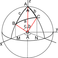
Consider three unit vectors OA, OB and OC drawn from the origin to the vertices of the triangle (on the unit sphere). The arc BC subtends an angle of magnitude a at the centre and therefore OB·OC=cos a. Introduce a Cartesian basis with OA along the z-axis and OB in the xz-plane making an angle c with the z-axis. The vector OC projects to ON in the xy-plane and the angle between ON and the x-axis is A. Therefore, the three vectors have components:

(0,\,0,\,1)

(\sin c,\,0,\,\cos c)

(\sin b\cos A,\,\sin b\sin A,\,\cos b)

The scalar product OB·OC in terms of the components is

OB·OC =

\sin c \,\sin b \, \cos A + \cos c \,\cos b

Equating the two expressions for the scalar product gives

\cos a = \cos b \,\cos c + \sin b \, \sin c \,\cos A.

This equation can be re-arranged to give explicit expressions for the angle in terms of the sides:

\cos A = \frac{\cos a\,-\,\cos b\,\cos c}{\sin b\, \sin c}.

The other cosine rules are obtained by cyclic permutations.

Derivation of the sine rule

This derivation is given in Todhunter,^[1] (Art.40). From the identity $\sin^2 A=1-\cos^2 A$ and the explicit expression for $\cos A$ given immediately above

\begin{align} \sin^2\!A &=1-\left(\frac{\cos a - \cos b\, \cos c}{\sin b \,\sin c}\right)^2\\ & =\frac{(1-\cos^2\!b)(1-\cos^2\!c)-(\cos a - \cos b\, \cos c)^2} {\sin^2\!b \,\sin^2\!c}\\ \frac{\sin A}{\sin a}&=\frac{[1-\cos^2\!a-\cos^2\!b-\cos^2\!c+2\cos a\cos b\cos c]^{1/2}}{\sin a\sin b\sin c}. \end{align}

Since the right hand side is invariant under a cyclic permutation of $a,\;b,\;c$ the spherical sine rule follows immediately. Banerjee ^[2] provides proofs using elementary linear algebra with the use of projection matrices.

Identities

Supplemental cosine rules

Applying the cosine rules to the polar triangle gives (Todhunter,^[1] Art.47), i.e. replacing A by π–a, a by π–A etc.,

\cos A = -\cos B \, \cos C + \sin B \, \sin C \, \cos a ,

\cos B = -\cos C \, \cos A + \sin C \, \sin A \, \cos b ,

\cos C = -\cos A \, \cos B + \sin A \, \sin B \, \cos c .

Cotangent four-part formulae

The six parts of a triangle may be written in cyclic order as (aCbAcB). The cotangent, or four-part, formulae relate two sides and two angles forming four consecutive parts around the triangle, for example (aCbA) or (BaCb). In such a set there are inner and outer parts: for example in the set (BaCb) the inner angle is C, the inner side is a, the outer angle is B, the outer side is b. The cotangent rule may be written as (Todhunter,^[1] Art.44)

\cos(\text{inner side}) \cos(\text{inner angle}) = \cot(\text{outer side}) \sin(\text{inner side})\ -\ \cot(\text{outer angle}) \sin(\text{inner angle}),

and the six possible equations are (with the relevant set shown at right):

\begin{array}{lll} \text{(CT1)}\quad& \cos b\,\cos C=\cot a\,\sin b - \cot A \,\sin C ,\qquad&(aCbA)\\[0ex] \text{(CT2)}& \cos b\,\cos A=\cot c\,\sin b - \cot C \,\sin A,&(CbAc)\\[0ex] \text{(CT3)}& \cos c\,\cos A=\cot b\,\sin c - \cot B \,\sin A,&(bAcB)\\[0ex] \text{(CT4)}& \cos c\,\cos B=\cot a\,\sin c - \cot A \,\sin B,&(AcBa)\\[0ex] \text{(CT5)}& \cos a\,\cos B=\cot c\,\sin a - \cot C \,\sin B,&(cBaC)\\[0ex] \text{(CT6)}& \cos a\,\cos C=\cot b\,\sin a - \cot B \,\sin C,&(BaCb). \end{array}

To prove the first formula start from the first cosine rule and on the right-hand side substitute for $\cos c$ from the third cosine rule:

\begin{align} \cos a & = \cos b \cos c + \sin b \sin c \cos A \\ & = \cos b\ (\cos a \cos b + \sin a \sin b \cos C ) + \sin b \sin C \sin a \cot A \\ \cos a \sin^2 b & = \cos b \sin a \sin b \cos C + \sin b \sin C \sin a \cot A. \end{align}

The result follows on dividing by $\sin a\sin b$ . Similar techniques with the other two cosine rules give CT3 and CT5. The other three equations follow by applying rules 1, 3 and 5 to the polar triangle.

Half-angle and half-side formulae

With $2s=(a+b+c)$ and $2S=(A+B+C)$ ,

\begin{align} & \sin{\textstyle\frac{1}{2}}A=\left[\frac{\sin(s{-}b)\sin(s{-}c)}{\sin b\sin c}\right]^{1/2} &\qquad &\sin{\textstyle\frac{1}{2}}a=\left[\frac{-\cos S\cos (S{-}A)}{\sin B\sin C}\right]^{1/2}\\[2ex] & \cos{\textstyle\frac{1}{2}}A=\left[\frac{\sin s\sin(s{-}a)}{\sin b\sin c}\right]^{1/2} &\qquad &\cos{\textstyle\frac{1}{2}}a=\left[\frac{\cos (S{-}B)\cos (S{-}C)}{\sin B\sin C}\right]^{1/2}\\[2ex] & \tan{\textstyle\frac{1}{2}}A=\left[\frac{\sin(s{-}b)\sin(s{-}c)}{\sin s\sin(s{-}a)}\right]^{1/2} &\qquad &\tan{\textstyle\frac{1}{2}}a=\left[\frac{-\cos S\cos (S{-}A)}{\cos (S{-}B)\cos(S{-}C)}\right]^{1/2} \end{align}

Another twelve identities follow by cyclic permutation.

The proof (Todhunter,^[1] Art.49) of the first formula starts from the identity 2sin²(A/2) = 1–cosA, using the cosine rule to express A in terms of the sides and replacing the sum of two cosines by a product. (See sum-to-product identities.) The second formula starts from the identity 2cos²(A/2) = 1+cosA, the third is a quotient and the remainder follow by applying the results to the polar triangle.

Delambre (or Gauss) analogies

\begin{align} &\\ \frac{\sin{\textstyle\frac{1}{2}}(A{+}B)} {\cos{\textstyle\frac{1}{2}}C} =\frac{\cos{\textstyle\frac{1}{2}}(a{-}b)} {\cos{\textstyle\frac{1}{2}}c} &\qquad\qquad & \frac{\sin{\textstyle\frac{1}{2}}(A{-}B)} {\cos{\textstyle\frac{1}{2}}C} =\frac{\sin{\textstyle\frac{1}{2}}(a{-}b)} {\sin{\textstyle\frac{1}{2}}c} \\[2ex] \frac{\cos{\textstyle\frac{1}{2}}(A{+}B)} {\sin{\textstyle\frac{1}{2}}C} =\frac{\cos{\textstyle\frac{1}{2}}(a{+}b)} {\cos{\textstyle\frac{1}{2}}c} &\qquad & \frac{\cos{\textstyle\frac{1}{2}}(A{-}B)} {\sin{\textstyle\frac{1}{2}}C} =\frac{\sin{\textstyle\frac{1}{2}}(a{+}b)} {\sin{\textstyle\frac{1}{2}}c} \end{align}

Another eight identities follow by cyclic permutation.

Proved by expanding the numerators and using the half angle formulae. (Todhunter,^[1] Art.54 and Delambre^[3])

Napier's analogies

\begin{align} &&\\[-2ex]\displaystyle {\tan{\textstyle\frac{1}{2}}(A{+}B)} =\frac{\cos{\textstyle\frac{1}{2}}(a{-}b)} {\cos{\textstyle\frac{1}{2}}(a{+}b)} \cot{\textstyle\frac{1}{2}C} &\qquad & {\tan{\textstyle\frac{1}{2}}(a{+}b)} =\frac{\cos{\textstyle\frac{1}{2}}(A{-}B)} {\cos{\textstyle\frac{1}{2}}(A{+}B)} \tan{\textstyle\frac{1}{2}c} \\[2ex] {\tan{\textstyle\frac{1}{2}}(A{-}B)} =\frac{\sin{\textstyle\frac{1}{2}}(a{-}b)} {\sin{\textstyle\frac{1}{2}}(a{+}b)} \cot{\textstyle\frac{1}{2}C} &\qquad & {\tan{\textstyle\frac{1}{2}}(a{-}b)} =\frac{\sin{\textstyle\frac{1}{2}}(A{-}B)} {\sin{\textstyle\frac{1}{2}}(A{+}B)} \tan{\textstyle\frac{1}{2}c} \end{align}

Another eight identities follow by cyclic permutation.

These identities follow by division of the Delambre formulae. (Todhunter,^[1] Art.52)

Napier's rules for right spherical triangles

When one of the angles, say C, of a spherical triangle is equal to π/2 the various identities given above are considerably simplified. There are ten identities relating three elements chosen from the set a, b, c, A, B.

Napier^[4] provided an elegant mnemonic aid for the ten independent equations: the mnemonic is called Napier's circle or Napier's pentagon (when the circle in the above figure, right, is replaced by a pentagon).

First write in a circle the six parts of the triangle (three vertex angles, three arc angles for the sides): for the triangle shown above left this gives aCbAcB. Next replace the parts that are not adjacent to C (that is A, c, B) by their complements and then delete the angle C from the list. The remaining parts are as shown in the above figure (right). For any choice of three contiguous parts, one (the middle part) will be adjacent to two parts and opposite the other two parts. The ten Napier's Rules are given by

sine of the middle part = the product of the tangents of the adjacent parts
sine of the middle part = the product of the cosines of the opposite parts

For an example, starting with the sector containing $a$ we have:

\sin a = \tan(\pi/2{-}B)\,\tan b = \cos(\pi/2{-}c)\, \cos(\pi/2{-}A) =\cot B\,\tan b = \sin c\,\sin A.

The full set of rules for the right spherical triangle is (Todhunter,^[1] Art.62)

\begin{alignat}{4} &\text{(R1)}&\qquad \cos c&=\cos a\,\cos b, &\qquad\qquad &\text{(R6)}&\qquad \tan b&=\cos A\,\tan c,\\ &\text{(R2)}& \sin a&=\sin A\,\sin c, &&\text{(R7)}& \tan a&=\cos B\,\tan c,\\ &\text{(R3)}& \sin b&=\sin B\,\sin c, &&\text{(R8)}& \cos A&=\sin B\,\cos a,\\ &\text{(R4)}& \tan a&=\tan A\,\sin b, &&\text{(R9)}& \cos B&=\sin A\,\cos b,\\ &\text{(R5)}& \tan b&=\tan B\,\sin a, &&\text{(R10)}& \cos c&=\cot A\,\cot B. \end{alignat}

Napier's rules for quadrantal triangles

A quadrantal spherical triangle together with Napier's circle for use in his mnemonics

When one of the sides, say c, of a spherical triangle is equal to π/2 the corresponding equations are obtained by applying the above rules to the polar triangle A'B'C' with sides a',b',c' such that A' = π–a, a' = π–A etc. This gives the following equations:

\begin{alignat}{4} &\text{(Q1)}&\qquad \cos C&=-\cos A\,\cos B, &\qquad\qquad &\text{(Q6)}&\qquad \tan B&=-\cos a\,\tan C,\\ &\text{(Q2)}& \sin A&=\sin a\,\sin C, &&\text{(Q7)}& \tan A&=-\cos b\,\tan C,\\ &\text{(Q3)}& \sin B&=\sin b\,\sin C, &&\text{(Q8)}& \cos a&=\sin b\,\cos A,\\ &\text{(Q4)}& \tan A&=\tan a\,\sin B, &&\text{(Q9)}& \cos b&=\sin a\,\cos B,\\ &\text{(Q5)}& \tan B&=\tan b\,\sin A, &&\text{(Q10)}& \cos C&=-\cot a\,\cot b. \end{alignat}

Five-part rules

Substituting the second cosine rule into the first and simplifying gives:

\cos a = (\cos a \,\cos c + \sin a \, \sin c \,\cos B) \cos c + \sin b \, \sin c \,\cos A

\cos a \,\sin^2 c = \sin a \,\cos c \,\sin c \,\cos B + \sin b \, \sin c \, \cos A

Cancelling the factor of $\sin c$ gives

\cos a \sin c = \sin a \,\cos c \, \cos B + \sin b \,\cos A

Similar substitutions in the other cosine and supplementary cosine formulae give a large variety of 5-part rules. They are rarely used.

Solution of triangles

Main article: Solution of triangles § Solving spherical triangles

Oblique triangles

The solution of triangles is the principal purpose of spherical trigonometry: given three, four or five elements of the triangle determine the remainder. The case of five given elements is trivial, requiring only a single application of the sine rule. For four given elements there is one non-trivial case, which is discussed below. For three given elements there are six cases: three sides, two sides and an included or opposite angle, two angles and an included or opposite side, or three angles. (The last case has no analogue in planar trigonometry.) No single method solves all cases. The figure below shows the seven non-trivial cases: in each case the given sides are marked with a cross-bar and the given angles with an arc. (The given elements are also listed below the triangle). There is a full discussion of the solution of oblique triangles in Todhunter^[1] (ChapterVI).

Case 1: three sides given. The cosine rule may be used to give the angles A, B, and C but, to avoid ambiguities, the half angle formulae are preferred.
Case 2: two sides and an included angle given. The cosine rule gives a and then we are back to Case 1.
Case 3: two sides and an opposite angle given. The sine rule gives C and then we have Case 7. There are either one or two solutions.
Case 4: two angles and an included side given. The four-part cotangent formulae for sets (cBaC) and (BaCb) give c and b, then A follows from the sine rule.
Case 5: two angles and an opposite side given. The sine rule gives b and then we have Case 7 (rotated). There are either one or two solutions.
Case 6: three angles given. The supplemental cosine rule may be used to give the sides a, b, and c but, to avoid ambiguities, the half-side formulae are preferred.
Case 7: two angles and two sides given. Use Napier's analogies for a and A.

The solution methods listed here are not the only possible choices: many others are possible. In general it is better to choose methods that avoid taking an inverse sine because of the possible ambiguity between an angle and its supplement. The use of half-angle formulae is often advisable because half-angles will be less than π/2 and therefore free from ambiguity. There is a full discussion in Todhunter. The solution of triangles article presents variants on these methods with a slightly different notation.

Solution by right-angled triangles

Another approach is to split the triangle into two right-angled triangles. For example, take the Case 3 example where b, c, B are given. Construct the great circle from A that is normal to the side BC at the point D. Use Napier's rules to solve the triangle ABD: use c and B to find the sides AD, BD and the angle BAD. Then use Napier's rules to solve the triangle ACD: that is use AD and b to find the side DC and the angles C and DAC. The angle A and side a follow by addition.

Numerical considerations

Not all of the rules obtained are numerically robust in extreme examples, for example when an angle approaches zero or π. Problems and solutions may have to be examined carefully, particularly when writing code to solve an arbitrary triangle.

Area and spherical excess

References

1 2 3 4 5 6 7 8 9 10 11 12 13 14 15 Todhunter, I. (1886). Spherical Trigonometry (5th ed.). MacMillan. This fifth edition is the cleanest available free version on the web The Gutenberg sources also include a latex version of the text. The latest (posthumous) and most complete version was published in 1911, co-authored with J. G. Leathem. The third edition has been issued by Amazon in paperback and Kindle versions . The text has been typeset but the formulae and diagrams have been pasted in as somewhat unsatisfactory images.
↑ Banerjee, Sudipto (2014), "Revisiting Spherical Trigonometry with Orthogonal Projectors", The College Mathematics Journal, Mathematical Association of America, 35: 375–381
↑ Delambre, J. B. J. (1807). Connaissance des Tems 1809. p. 445.
↑ Napier, J (1614). Mirifici Logarithmorum Canonis Constructio. p. 50. An 1889 translation The Construction of the Wonderful Canon of Logarithms is available as en e-book from Abe Books
↑ Another proof of Girard's theorem may be found at .
↑ Rapp, Richard. H (1991). Geometric Geodesy Part I (PDF). p. 89. (pdf page 99),
↑ Clarke, Alexander Ross (1880). Geodesy. Clarendon Press. (Chapters 2 and 9). Recently republished at Forgotten Books

External links

Wolfram's mathworld: Spherical Trigonometry a more thorough list of identities, with some derivation
Wolfram's mathworld: Spherical Triangle nice applet
TriSph A free software to solve the spherical triangles, configurable to different practical applications and configured for gnomonic
"Revisiting Spherical Trigonometry with Orthogonal Projectors" by Sudipto Banerjee. The paper derives the spherical law of cosines and law of sines using elementary linear algebra and projection matrices.
A Visual Proof of Girard's Theorem by Okay Arik, the Wolfram Demonstrations Project.
"The Book of Instruction on Deviant Planes and Simple Planes" is a manuscript in Arabic that dates back to 1740 and talks about spherical trigonometry, with diagrams.
Some Algorithms for Polygons on a Sphere Robert G. Chamberlain, William H. Duquette, Jet Propulsion Laboratory. The paper develops and explains many useful formulae, perhaps with a focus on navigation and cartography.
Online computation of spherical triangles

Authority control	NDL: 00570155

This article is issued from Wikipedia - version of the 11/30/2016. The text is available under the Creative Commons Attribution/Share Alike but additional terms may apply for the media files.