Multidelay block frequency domain adaptive filter
The Multidelay block frequency domain adaptive filter (MDF) algorithm is a block-based frequency domain implementation of the (normalised) Least mean squares filter (LMS) algorithm.
Introduction
The MDF algorithm is based on the fact that convolutions may be efficiently computed in the frequency domain (thanks to the Fast Fourier Transform). However, the algorithm differs from the Fast LMS algorithm in that block size it uses may be smaller than the filter length. If both are equal, then MDF reduces to the FLMS algorithm.
The advantages of MDF over the (N)LMS algorithm are:
- Lower algorithmic complexity
- Partial de-correlation of the input (which 'may' lead to faster convergence)
Variable definitions

Let  be the length of the processing blocks,
  be the number of blocks and
  denote the 2Nx2N Fourier transform matrix. The variables are defined as:
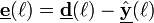
![\underline{\mathbf{e}}(\ell) = \mathbf{F}\left[ \mathbf{0}_{1xN}, e(\ell N),\dots,e(\ell N-N-1) \right]^T](../I/m/63e712b58032fbb1cfdb43afe8172de6.png)
![\underline{\mathbf{x}}_k(\ell) = \mathrm{diag} \left\{ \mathbf{F}\left[ x((\ell -k+1) N),\dots,x((\ell -k-1) N-1) \right]^T \right\}](../I/m/40a4e2b16088be1ee07df62f91f73009.png)
![\underline{\mathbf{X}}(\ell) = \left[ \underline{\mathbf{x}}_0(\ell), \underline{\mathbf{x}}_1(\ell), \dots, \underline{\mathbf{x}}_{K-1}(\ell) \right]](../I/m/f13fc3952fb92a7e42f823aa4c90af00.png)
![\underline{\mathbf{d}}(\ell) = \mathbf{F}\left[ \mathbf{0}_{1xN}, d(\ell N),\dots,d(\ell N-N-1) \right]^T](../I/m/79e54606ed320c0dccb5311cb1efa3de.png)
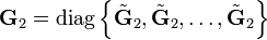
With normalisation matrices  and
and  :
:


In practice, when multiplying a column vector  by , we take the inverse FFT of , set the first values in the result to zero and then take the FFT. This is meant to remove the effects of the circular convolution.
Algorithm description
For each block, the MDF algorithm is computed as:


It is worth noting that, while the algorithm is more easily expressed in matrix form, the actual implementation requires no matrix multiplications. For instance the normalisation matrix computation  reduces to an element-wise vector multiplication because
  is block-diagonal. The same goes for other multiplications.
References
- J.-S. Soo and K. Pang, “Multidelay block frequency domain adaptive filter,” IEEE Transactions on Acoustics, Speech and Signal Processing, vol. 38, no. 2, pp. 373–376, 1990.
- H. Buchner, J. Benesty, W. Kellermann, "An Extended Multidelay Filter: Fast Low-Delay Algorithms for Very High-Order Adaptive Systems". Proc. IEEE International Conference on Acoustics, Speech, and Signal Processing (ICASSP), 2003.
- A free implementation of the MDF algorithm is available in Speex (main source file)
See also
- Adaptive filter
- Recursive least squares
- For statistical techniques relevant to LMS filter see Least squares.