Monotone cubic interpolation

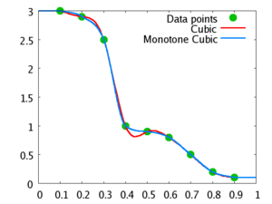
In the mathematical subfield of numerical analysis, monotone cubic interpolation is a variant of cubic interpolation that preserves monotonicity of the data set being interpolated.

Monotonicity is preserved by linear interpolation but not guaranteed by cubic interpolation.

Monotone cubic Hermite interpolation

Example showing non-monotone cubic interpolation (in red) and monotone cubic interpolation (in blue) of a monotone data set.

Monotone interpolation can be accomplished using cubic Hermite spline with the tangents $m_{i}$ modified to ensure the monotonicity of the resulting Hermite spline.

An algorithm is also available for monotone quintic Hermite interpolation.

Interpolant selection

There are several ways of selecting interpolating tangents for each data point. This section will outline the use of the Fritsch–Carlson method.

Let the data points be $(x_k,y_k)$ for $k=1,...,n$

Compute the slopes of the secant lines between successive points:
$\Delta_k =\frac{y_{k+1}-y_k}{x_{k+1}-x_k}$
for $k=1,\dots,n-1$ .
Initialize the tangents at every data point as the average of the secants,
$m_k = \frac{\Delta_{k-1}+\Delta_k}{2}$
for $k=2,\dots,n-1$ ; if $\Delta _{{k-1}}$ and $\Delta _{k}$ have different sign, set $m_{k}=0$ . These may be updated in further steps. For the endpoints, use one-sided differences:
$m_1 = \Delta_1 \quad \text{and} \quad m_n = \Delta_{n-1}$
For $k=1,\dots,n-1$ , if $\Delta_k = 0$ (if two successive $y_k=y_{k+1}$ are equal), then set $m_k = m_{k+1} = 0,$ as the spline connecting these points must be flat to preserve monotonicity. Ignore step 4 and 5 for those $k$ .
Let $\alpha_k = m_k/\Delta_k$ and $\beta_k = m_{k+1}/\Delta_k$ . If $\alpha _{k}$ or $\beta_{k-1}$ are computed to be less than zero, then the input data points are not strictly monotone, and $(x_k,y_k)$ is a local extremum. In such cases, piecewise monotone curves can still be generated by choosing $m_{k}=0$ , although global strict monotonicity is not possible.
To prevent overshoot and ensure monotonicity, at least one of the following conditions must be met:
1. the function
  $\phi(\alpha, \beta) = \alpha - \frac{(2 \alpha + \beta - 3)^2}{3(\alpha + \beta - 2)}$
  must have a value greater than or equal to zero;
2. $\alpha + 2\beta - 3 \le 0$ ; or
3. $2\alpha + \beta - 3 \le 0$ .

If monotonicity must be strict then $\phi(\alpha, \beta)$ must have a value strictly greater than zero.

One simple way to satisfy this constraint is to restrict the magnitude of vector $(\alpha_k, \beta_k)$ to a circle of radius 3. That is, if $\alpha_k^2 + \beta_k^2 > 9$ , then set $m_k = \tau_k \alpha_k \Delta_k$ and $m_{k+1} = \tau_k \beta_k \Delta_k$ where $\tau_k = \frac{3}{\sqrt{\alpha_k^2 + \beta_k^2}}$ .

Alternatively it is sufficient to restrict $\alpha_k \le 3$ and $\beta_k \le 3$ . To accomplish this if $\alpha_k > 3$ , then set $m_k = 3\times \Delta_k$ . Similarly for $\beta$ .

Note that only one pass of the algorithm is required.

Cubic interpolation

After the preprocessing, evaluation of the interpolated spline is equivalent to cubic Hermite spline, using the data $x_{k}$ , $y_{k}$ , and $m_{k}$ for $k=1,...,n$ .

To evaluate at $x$ , find the smallest value larger than $x$ , $x_\text{upper}$ , and the largest value smaller than $x$ , $x_\text{lower}$ , among $x_{k}$ such that $x_\text{lower} \leq x \leq x_\text{upper}$ . Calculate

h = x_\text{upper}-x_\text{lower}

and

t = \frac{x - x_\text{lower}}{h}

then the interpolant is

f_\text{interpolated}(x) = y_\text{lower} h_{00}(t) + h m_\text{lower} h_{10}(t) + y_\text{upper} h_{01}(t) + h m_\text{upper}h_{11}(t)

where $h_{ii}$ are the basis functions for the cubic Hermite spline.

Example implementation

The following JavaScript implementation takes a data set and produces a monotone cubic spline interpolant function:

/* Monotone cubic spline interpolation
   Usage example:
	var f = createInterpolant([0, 1, 2, 3, 4], [0, 1, 4, 9, 16]);
	var message = '';
	for (var x = 0; x <= 4; x += 0.5) {
		var xSquared = f(x);
		message += x + ' squared is about ' + xSquared + '\n';
	}
	alert(message);
*/
var createInterpolant = function(xs, ys) {
	var i, length = xs.length;
	
	// Deal with length issues
	if (length != ys.length) { throw 'Need an equal count of xs and ys.'; }
	if (length === 0) { return function(x) { return 0; }; }
	if (length === 1) {
		// Impl: Precomputing the result prevents problems if ys is mutated later and allows garbage collection of ys
		// Impl: Unary plus properly converts values to numbers
		var result = +ys[0];
		return function(x) { return result; };
	}
	
	// Rearrange xs and ys so that xs is sorted
	var indexes = [];
	for (i = 0; i < length; i++) { indexes.push(i); }
	indexes.sort(function(a, b) { return xs[a] < xs[b] ? -1 : 1; });
	var oldXs = xs, oldYs = ys;
	// Impl: Creating new arrays also prevents problems if the input arrays are mutated later
	xs = []; ys = [];
	// Impl: Unary plus properly converts values to numbers
	for (i = 0; i < length; i++) { xs.push(+oldXs[indexes[i]]); ys.push(+oldYs[indexes[i]]); }
	
	// Get consecutive differences and slopes
	var dys = [], dxs = [], ms = [];
	for (i = 0; i < length - 1; i++) {
		var dx = xs[i + 1] - xs[i], dy = ys[i + 1] - ys[i];
		dxs.push(dx); dys.push(dy); ms.push(dy/dx);
	}
	
	// Get degree-1 coefficients
	var c1s = [ms[0]];
	for (i = 0; i < dxs.length - 1; i++) {
		var m = ms[i], mNext = ms[i + 1];
		if (m*mNext <= 0) {
			c1s.push(0);
		} else {
			var dx_ = dxs[i], dxNext = dxs[i + 1], common = dx_ + dxNext;
			c1s.push(3*common/((common + dxNext)/m + (common + dx_)/mNext));
		}
	}
	c1s.push(ms[ms.length - 1]);
	
	// Get degree-2 and degree-3 coefficients
	var c2s = [], c3s = [];
	for (i = 0; i < c1s.length - 1; i++) {
		var c1 = c1s[i], m_ = ms[i], invDx = 1/dxs[i], common_ = c1 + c1s[i + 1] - m_ - m_;
		c2s.push((m_ - c1 - common_)*invDx); c3s.push(common_*invDx*invDx);
	}
	
	// Return interpolant function
	return function(x) {
		// The rightmost point in the dataset should give an exact result
		var i = xs.length - 1;
		if (x == xs[i]) { return ys[i]; }
		
		// Search for the interval x is in, returning the corresponding y if x is one of the original xs
		var low = 0, mid, high = c3s.length - 1;
		while (low <= high) {
			mid = Math.floor(0.5*(low + high));
			var xHere = xs[mid];
			if (xHere < x) { low = mid + 1; }
			else if (xHere > x) { high = mid - 1; }
			else { return ys[mid]; }
		}
		i = Math.max(0, high);
		
		// Interpolate
		var diff = x - xs[i], diffSq = diff*diff;
		return ys[i] + c1s[i]*diff + c2s[i]*diffSq + c3s[i]*diff*diffSq;
	};
};

References

Fritsch, F. N.; Carlson, R. E. (1980). "Monotone Piecewise Cubic Interpolation". SIAM Journal on Numerical Analysis. SIAM. 17 (2): 238–246. doi:10.1137/0717021.
Dougherty, R.L.; Edelman, A.; Hyman, J.M. (April 1989). "Positivity-, monotonicity-, or convexity-preserving cubic and quintic Hermite interpolation". Mathematics of Computation. 52 (186): 471–494. doi:10.2307/2008477.

External links

GPLv3 licensed C++ implementation: MonotCubicInterpolator.cpp MonotCubicInterpolator.hpp

This article is issued from Wikipedia - version of the 5/14/2016. The text is available under the Creative Commons Attribution/Share Alike but additional terms may apply for the media files.