Midpoint method

For the midpoint rule in numerical quadrature, see rectangle method.

Illustration of the midpoint method assuming that

y_{n}

equals the exact value

y(t_n).

The midpoint method computes

y_{n+1}

so that the red chord is approximately parallel to the tangent line at the midpoint (the green line).

In numerical analysis, a branch of applied mathematics, the midpoint method is a one-step method for numerically solving the differential equation,

y'(t) = f(t, y(t)), \quad y(t_0) = y_0

The explicit midpoint method is given by the formula

y_{n+1} = y_n + hf\left(t_n+\frac{h}{2},y_n+\frac{h}{2}f(t_n, y_n)\right), \qquad\qquad (1e)

the implicit midpoint method by

y_{n+1} = y_n + hf\left(t_n+\frac{h}{2},\frac12 (y_n+y_{n+1})\right), \qquad\qquad (1i)

for $n=0, 1, 2, \dots$ Here, $h$ is the step size — a small positive number, $t_n=t_0 + n h,$ and $y_{n}$ is the computed approximate value of $y(t_n).$ The explicit midpoint method is also known as the modified Euler method,^[1] the implicit method is the most simple collocation method, and, applied to Hamiltionian dynamics, a symplectic integrator.

The name of the method comes from the fact that in the formula above the function $f$ giving the slope of the solution is evaluated at $t=t_n+h/2,$ which is the midpoint between $t_{n}$ at which the value of y(t) is known and $t_{n+1}$ at which the value of y(t) needs to be found.

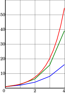
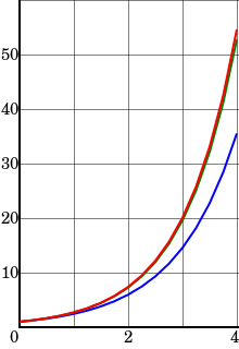
The local error at each step of the midpoint method is of order $O\left(h^3\right)$ , giving a global error of order $O\left(h^2\right)$ . Thus, while more computationally intensive than Euler's method, the midpoint method's error generally decreases faster as $h \to 0$ .

The methods are examples of a class of higher-order methods known as Runge-Kutta methods.

Derivation of the midpoint method

Illustration of numerical integration for the equation

y'=y,y(0)=1.

Blue: the Euler method, green: the midpoint method, red: the exact solution,

y=e^{t}.

The step size is

h=1.0.

The same illustration for

h=0.25.

It is seen that the midpoint method converges faster than the Euler method.

The midpoint method is a refinement of the Euler's method

y_{n+1} = y_n + hf(t_n,y_n),\,

and is derived in a similar manner. The key to deriving Euler's method is the approximate equality

y(t+h) \approx y(t) + hf(t,y(t)) \qquad\qquad (2)

which is obtained from the slope formula

y'(t) \approx \frac{y(t+h) - y(t)}{h} \qquad\qquad (3)

and keeping in mind that $y' = f(t, y).$

For the midpoint methods, one replaces (3) with the more accurate

y'\left(t+\frac{h}{2}\right) \approx \frac{y(t+h) - y(t)}{h}

when instead of (2) we find

y(t+h) \approx y(t) + hf\left(t+\frac{h}{2},y\left(t+\frac{h}{2}\right)\right). \qquad\qquad (4)

One cannot use this equation to find $y(t+h)$ as one does not know $y$ at $t+h/2$ . The solution is then to use a Taylor series expansion exactly as if using the Euler method to solve for $y(t+h/2)$ :

y\left(t + \frac{h}{2}\right) \approx y(t) + \frac{h}{2}y'(t)=y(t) + \frac{h}{2}f(t, y(t)),

which, when plugged in (4), gives us

y(t + h) \approx y(t) + hf\left(t + \frac{h}{2}, y(t) + \frac{h}{2}f(t, y(t))\right)

and the explicit midpoint method (1e).

The implicit method (1i) is obtained by approximating the value at the half step $t+h/2$ by the midpoint of the line segment from $y(t)$ to $y(t+h)$

y\left(t+\frac h2\right)\approx \frac12\bigl(y(t)+y(t+h)\bigr)

and thus

\frac{y(t+h)-y(t)}{h}\approx y'\left(t+\frac h2\right)\approx k=f\left(t+\frac h2,\frac12\bigl(y(t)+y(t+h)\bigr)\right)

Inserting the approximation $y_n+h\,k$ for $y(t_n+h)$ results in the implicit Runge-Kutta method

\begin{align} k&=f\left(t_n+\frac h2,y_n+\frac h2 k\right)\\ y_{n+1}&=y_n+h\,k \end{align}

which contains the implicit Euler method with step size $h/2$ as its first part.

Because of the time symmetry of the implicit method, all terms of even degree in $h$ of the local error cancel, so that the local error is automatically of order $\mathcal O(h^3)$ . Replacing the implicit with the explicit Euler method in the determination of $k$ results again in the explicit midpoint method.

Notes

↑ Süli & Mayers 2003, p. 328

References

Griffiths,D. V.; Smith, I. M. (1991). Numerical methods for engineers: a programming approach. Boca Raton: CRC Press. p. 218. ISBN 0-8493-8610-1.
Süli, Endre; Mayers, David (2003), An Introduction to Numerical Analysis, Cambridge University Press, ISBN 0-521-00794-1 .

Numerical methods for integration

First-order methods	Euler method Backward Euler Semi-implicit Euler Exponential Euler

Second-order methods	Verlet integration Velocity Verlet Trapezoidal rule Beeman's algorithm Midpoint method Heun's method Newmark-beta method Leapfrog integration

Higher-order methods	Exponential integrators Runge–Kutta methods List of Runge–Kutta methods Linear multistep method General linear methods Backward differentiation formula

This article is issued from Wikipedia - version of the 6/3/2016. The text is available under the Creative Commons Attribution/Share Alike but additional terms may apply for the media files.

Midpoint method

Derivation of the midpoint method

See also

Notes

References