Medcouple

A histogram of 5000 random values sampled from a skew gamma distribution above, and the corresponding histogram of the medcouple kernel values below. The actual medcouple is the median of the bottom distribution, marked at 0.188994 with a yellow line.

The medcouple is a robust statistic that measures the skewness of a univariate distribution.^[1] Its robustness makes it suitable for identifying outliers in adjusted boxplots.^[2]^[3] Ordinary boxplots do not fare well with skew distributions, since they label the longer unsymmetrical tails as outliers. Using the medcouple, the whiskers of a boxplot can be adjusted for skew distributions and thus have a more accurate identification of outliers for non-symmetrical distributions.

As a kind of order statistic, the medcouple belongs to the class of incomplete generalised L-statistics.^[1] Like the ordinary median or mean, the medcouple is a nonparametric statistic, thus it can be computed for any distribution.

Definition

In order to harmonise with zero-based indexing in many programming languages, we will index from zero in all that follows.

Let $X:=x_{0}\geq x_{1}\geq \ldots \geq x_{{n-1}}$ be an ordered sample of size $n$ , and let $x_{m}$ be the median of $X$ . Define the sets

X^{+}:=\{x_{i}~|~x_{i}\geq x_{m}\}

X^{-}:=\{x_{j}~|~x_{j}\leq x_{m}\}

of sizes $p:=|X^{+}|$ and $q:=|X^{-}|$ respectively. For $x_{i}^{+}\in X^{+}$ and $x_{j}^{-}\in X^{-}$ , we define the kernel function

h(x_{i}^{+},x_{j}^{-}):={\begin{cases}\displaystyle {\frac {(x_{i}^{+}-x_{m})-(x_{m}-x_{j}^{-})}{x_{i}^{+}-x_{j}^{-}}}&{\text{ if }}x_{i}^{+}>x_{j}^{-},\\\operatorname {signum}(p-1-i-j)&{\text{ if }}x_{i}^{+}=x_{m}=x_{j}^{-},\end{cases}}

where $\operatorname {signum}$ is the sign function.

The medcouple is then the median of the set^[1]^:998

\{h(x_{i}^{+},x_{j}^{-})~|~x_{i}^{+}\in X^{+}{\text{ and }}x_{j}^{-}\in X^{-}\}

In other words, we split the distribution into all values greater or equal to the median and all values less than or equal to the median. We define a kernel function whose first variable is over the $p$ greater values and whose second variable is over the $q$ lesser values. For the special case of values tied to the median, we define the kernel by the signum function. The medcouple is then the median over all $pq$ values of $h(x_{i}^{+},x_{j}^{-})$ .

Since the medcouple is not a median applied to all $(x_{i},x_{j})$ couples, but only to those for which $x_{i}^{+}\geq x_{m}\geq x_{j}^{-}$ , it belongs to the class of incomplete generalised L-statistics.^[1]^:998

Properties of the medcouple

The medcouple has a number of desirable properties. A few of them are directly inherited from the kernel function.

The medcouple kernel

We make the following observations about the kernel function $h(x_{i}^{+},x_{j}^{-})$ :

The kernel function is location-invariant.^[1]^:999 If we add or subtract any value to each element of the sample $X$ , the corresponding values of the kernel function do not change.
The kernel function is scale-invariant.^[1]^:999 Equally scaling all elements of the sample $X$ does not alter the values of the kernel function.

These properties are in turn inherited by the medcouple. Thus, the medcouple is independent of the mean and standard deviation of a distribution, a desirable property for measuring skewness. For ease of computation, these properties enable us to define the two sets

Z^{+}:=\left.\left\{{\frac {x_{i}^{+}-x_{m}}{r}}~\right|~x_{i}^{+}\in X^{+}\right\}

Z^{-}:=\left.\left\{{\frac {x_{j}^{-}-x_{m}}{r}}~\right|~x_{j}^{-}\in X^{-}\right\}

where $r=2\max _{{0\leq i\leq n-1}}|x_{i}|$ . This makes the set $Z:=Z^{+}\cup Z^{-}$ have range of at most 1, median 0, and keep the same medcouple as $X$ .

For $Z$ , the medcouple kernel reduces to

h(z_{i}^{+},z_{j}^{-}):={\begin{cases}\displaystyle {\frac {z_{i}^{+}+z_{j}^{-}}{z_{i}^{+}-z_{j}^{-}}}&{\text{ if }}z_{i}^{+}>z_{j}^{-}\\\operatorname {signum}(p-1-i-j)&{\text{ if }}z_{i}^{+}=0=z_{j}^{-}\end{cases}}

Using the recentred and rescaled set $Z$ we can observe the following.

The kernel function is between -1 and 1,^[1]^:998 that is, $|h(z_{i}^{+},z_{j}^{-})|\leq 1$ . This follows from the reverse triangle inequality $|a|-|b|\leq |a-b|$ with $a=z_{i}^{+}$ and $b=z_{j}^{-}$ and the fact that $z_{i}^{+}\geq 0\geq z_{j}^{-}$ .
The medcouple kernel $h(z_{i}^{+},z_{j}^{-})$ is non-decreasing in each variable.^[1]^:1005 This can be verified by the partial derivatives ${\frac {\partial h}{\partial z_{i}^{+}}}$ and ${\frac {\partial h}{\partial z_{j}^{-}}}$ , both nonnegative, since $z_{i}^{+}\geq 0\geq z_{j}^{-}$ .

With properties 1, 2, and 4, we can thus define the following matrix,

H:=(h_{{ij}})=(h(z_{i}^{+},z_{j}^{-}))={\begin{pmatrix}h(z_{0}^{+},z_{0}^{-})&\cdots &h(z_{0}^{+},z_{{q-1}}^{-})\\\vdots &\ddots &\vdots \\h(z_{{p-1}}^{+},z_{0}^{-})&\cdots &h(z_{{p-1}}^{+},z_{{q-1}}^{-})\end{pmatrix}}.

If we sort the sets $Z^{+}$ and $Z^{-}$ in decreasing order, then the matrix $H$ has sorted rows and sorted columns,^[1]^:1006

H={\begin{pmatrix}h(z_{0}^{+},z_{0}^{-})&\geq &\cdots &\geq &h(z_{0}^{+},z_{{q-1}}^{-})\\\geq &&&&\geq \\\vdots &&\ddots &&\vdots \\\geq &&&&\geq \\h(z_{{p-1}}^{+},z_{0}^{-})&\geq &\cdots &\geq &h(z_{{p-1}}^{+},z_{{q-1}}^{-})\end{pmatrix}}.

The medcouple is then the median of this matrix with sorted rows and sorted columns. The fact that the rows and columns are sorted allows the implementation of a fast algorithm for computing the medcouple.

Robustness

The breakdown point is the number of values that a statistic can resist before it becomes meaningless, i.e. the number of arbitrarily large outliers that the data set $X$ may have before the value of the statistic is affected. For the medcouple, the breakdown point is 25%, since it is a median taken over the couples $(x_{i},x_{j})$ such that $x_{i}\geq x_{m}\geq x_{j}$ .^[1]^:1002

Values

Like all measures of skewness, the medcouple is positive for distributions that are skewed to the right, negative for distributions skewed to the left, and zero for symmetrical distributions. In addition, the values of the medcouple are bounded by 1 in absolute value.^[1]^:998

Algorithms for computing the medcouple

Before presenting medcouple algorithms, we recall that there exist $O(n)$ algorithms for the finding the median. Since the medcouple is a median, ordinary algorithms for median-finding are important.

Naïve algorithm

The naïve algorithm for computing the medcouple is slow.^[1]^:1005 It proceeds in two steps. First, it constructs the medcouple matrix $H$ which contains all of the possible values of the medcouple kernel. In the second step, it finds the median of this matrix. Since there are $pq\approx {\frac {n^{2}}{4}}$ entries in the matrix in the case when all elements of the data set $X$ are unique, the algorithmic complexity of the naïve algorithm is $O(n^{2})$ .

More concretely, the naïve algorithm proceeds as follows. Recall that we are using zero-based indexing.


   function naïve_medcouple(vector X):
       // X is a vector of size n.
       
       //Sorting in decreasing order can be done in-place in O(n log n) time
       sort_decreasing(X)
       
       xm := median(X)
       xscale := 2*max(X)
       
       // define the upper and lower centred and rescaled vectors
       // they inherit X's own decreasing sorting
       Zplus  := [(x - xm)/xscale | x in X such that x >= xm]
       Zminus := [(x - xm)/xscale | x in X such that x <= xm]
       
       p := size(Zplus)
       q := size(Zminus)
       
       // define the kernel function closing over Zplus and Zminus
       function h(i,j):
           a := Zplus[i]
           b := Zminus[j]
           
           if a == b:
               return signum(p - 1 - i - j)
           else:
               return (a + b)/(a - b)
           endif
       endfunction
       
       // O(n^2) operations necessary to form this vector
       H := [h(i,j) | i in [0, 1, ..., p - 1] and j in [0, 1, ..., q - 1]]
       
       return median(H)
   endfunction

The final call to median on a vector of size $O(n^{2})$ can be done itself in $O(n^{2})$ operations, hence the entire naïve medcouple algorithm is of the same complexity.

Fast algorithm

The fast algorithm outperforms the naïve algorithm by exploiting the sorted nature of the medcouple matrix $H$ . Instead of computing all entries of the matrix, the fast algorithm uses the K^th pair algorithm of Johnson & Mizoguchi.^[4]

The first stage of the fast algorithm proceeds as the naïve algorithm. We first compute the necessary ingredients for the kernel matrix, $H=(h_{{ij}})$ , with sorted rows and sorted columns in decreasing order. Rather than computing all values of $h_{ij}$ , we instead exploit the monotonicity in rows and columns, via the following observations.

Comparing a value against the kernel matrix

First, we note that we can compare any $u$ with all values $h_{ij}$ of $H$ in $O(n)$ time.^[4]^:150 For example, for determining all $i$ and $j$ such that $h_{{ij}}>u$ , we have the following function:

    function greater_h(kernel h, int p, int q, real u):
        // h is the kernel function, h(i,j) gives the ith, jth entry of H
        // p and q are the number of rows and columns of the kernel matrix H
        
        // vector of size p
        P := vector(p)
        
        // indexing from zero
        j := 0
        
        // starting from the bottom, compute the least upper bound for each row
        for i := p - 1, p - 2, ..., 1, 0:
                 
            // search this row until we find a value less than u
            while j < q and h(i, j) > u:
                j := j + 1
            endwhile
            
            // the entry preceding the one we just found is greater than u
            P[i] := j - 1
        endfor
        
        return P
    endfunction

This greater_h function is traversing the kernel matrix from the bottom left to the top right, and returns a vector $P$ of indices that indicate for each row where the boundary lies between values greater than $u$ and those less than or equal to $u$ . This method works because of the row-column sorted property of $H=(h_{{ij}})$ . Since greater_h computes at most $p + q$ values of $h_{ij}$ , its complexity is $O(n)$ .^[4]^:150

Conceptually, the resulting $P$ vector can be visualised as establishing a boundary on the matrix as suggested by the following diagram, where the red entries are all larger than $u$ :

The symmetric algorithm for computing the values of $h_{ij}$ less than $u$ is very similar. It instead proceeds along $H$ in the opposite direction, from the top right to the bottom left:

    function less_h(kernel h, int p, int q, real u):
    
        // vector of size p
        Q := vector(p)
        
        // last possible row index
        j := q - 1
        
        // starting from the top, compute the greatest lower bound for each row
        for i := 0, 1, ..., p - 2, p - 1:
        
            // search this row until we find a value greater than u
            while j >= 0 and h(i, j) < u:
                j := j - 1
            endwhile
            
            // the entry following the one we just found is less than u
            Q[i] := j + 1
        endfor
        
        return Q
    endfunction

This lower boundary can be visualised like so, where the blue entries are smaller than $u$ :

For each $i$ , we have that $P_{i}\geq Q_{i}$ , with strict inequality occurring only for those rows that have values equal to $u$ .

We also have that the sums

\sum _{{i=0}}^{{p-1}}(P_{i}+1)~\qquad ~\sum _{{i=0}}^{{p-1}}Q_{i}

give, respectively, the number of elements of $H$ that are greater than $u$ , and the number of elements that are greater than or equal to $u$ . Thus this method also yields the rank of $u$ within the elements $h_{ij}$ of $H$ .^[4]^:149

Weighted median of row medians

The second observation is that we can use the sorted matrix structure to instantly compare any element to at least half of the entries in the matrix. For example, the median of the row medians across the entire matrix is less than the upper left quadrant in red, but greater than the lower right quadrant in blue:

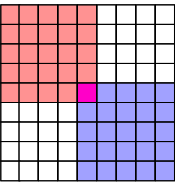
More generally, using the boundaries given by the $P$ and $Q$ vectors from the previous section, we can assume that after some iterations, we have pinpointed the position of the medcouple to lie between the red left boundary and the blue right boundary:^[4]^:149

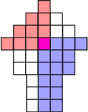
The yellow entries indicate the median of each row. If we mentally re-arrange the rows so that the medians align and ignore the discarded entries outside the boundaries,

we can select a weighted median of these medians, each entry weighted by the number of remaining entries on this row. This ensures that we can discard at least 1/4 of all remaining values no matter if we have to discard the larger values in red or the smaller values in blue:

Each row median can be computed in $O(1)$ time, since the rows are sorted, and the weighted median can be computed in $O(n)$ time, using a binary search.^[4]^:148

K^th pair algorithm

A visualisation of the fast medcouple algorithm. It begins with a matrix with sorted rows and sorted columns, where darker squares are smaller than lighter squares. At each iteration, the weighted median of row medians is picked, in yellow. It is then compared to the rest of the matrix to produce candidate red upper and blue lower boundaries. The algorithm then selects the boundary which is known to exclude the global matrix median, by considering the number of entries excluded by this boundary (which is equivalent to considering the rank of the yellow entry). The algorithm then proceeds until the yellow weighted median of row medians is exactly the medcouple, or the number of candidate entries is small enough to perform a selection sort amongst the remaining entries.

Putting together these two observations, the fast medcouple algorithm proceeds broadly as follows.^[4]^:148

Compute the necessary ingredients for the medcouple kernel function $h(i,j)$ with $p$ sorted rows and $q$ sorted columns.
At each iteration, approximate the medcouple with the weighted median of the row medians.^[4]^:148
Compare this tentative guess to the entire matrix obtaining right and left boundary vectors $P$ and $Q$ respectively. The sum of these vectors also gives us the rank of this tentative medcouple.
1. If the rank of the tentative medcouple is exactly $pq/2$ , then stop. We have found the medcouple.
2. Otherwise, discard the entries greater than or less than the tentative guess by picking either $P$ or $Q$ as the new right or left boundary, depending on which side the element of rank $pq/2$ is in. This step always discards at least 1/4 of all remaining entries.
Once the number of candidate medcouples between the right and left boundaries is less than or equal to $p$ , perform a rank selection amongst the remaining entries, such that the rank within this smaller candidate set corresponds to the $pq/2$ rank of the medcouple within the whole matrix.

The initial sorting in order to form the $h(i,j)$ function takes $O(n\log n)$ time. At each iteration, the weighted median takes $O(n)$ time, as well as the computations of the new tentative $P$ and $Q$ left and right boundaries. Since each iteration discards at least 1/4 of all remaining entries, there will be at most $O(\log n)$ iterations.^[4]^:150 Thus, the whole fast algorithm takes $O(n\log n)$ time.^[4]^:150

Let us restate the fast algorithm in more detail.


   function medcouple(vector X):
       // X is a vector of size n
       
       // compute initial ingredients as for the naïve medcouple
       sort_decreasing(X)
       
       xm := median(X)
       xscale := 2*max(X)
       
       Zplus  := [(x - xm)/xscale | x in X such that x >= xm]
       Zminus := [(x - xm)/xscale | x in X such that x <= xm]
       
       p := size(Zplus)
       q := size(Zminus)
       
       function h(i,j):
           a := Zplus[i]
           b := Zminus[j]
           
           if a == b:
               return signum(p - 1 - i - j)
           else:
               return (a + b)/(a - b)
           endif
       endfunction
       
       // begin Kth pair algorithm (Johnson & Mizoguchi)
       
       // the initial left and right boundaries, two vectors of size p
       L := [0, 0, ..., 0]
       R := [q - 1, q - 1, ..., q - 1]
       
       // number of entries to the left of the left boundary
       Ltotal := 0
       
       // number of entries to the left of the right boundary
       Rtotal := p*q
       
       // since we are indexing from zero, the medcouple index is one
       // less than its rank
       medcouple_index := floor(Rtotal/2)
       
       // iterate while the number of entries between the boundaries is
       // greater than the number of rows in the matrix
       while Rtotal - Ltotal > p:
           
           // compute row medians and their associated weights, but skip
           // any rows that are already empty
           middle_idx  := [i | i in [0, 1, ..., p - 1] such that L[i] <= R[i]]
           row_medians := [h(i, floor((L[i] + R[i])/2) | i in middle_idx]
           weights := [R[i] - L[i] + 1 | i in middle_idx]
           
           WM := weighted median(row_medians, weights)
           
           // new tentative right and left boundaries
           P := greater_h(h, p, q, WM)
           Q := less_h(h, p, q, WM)
           
           Ptotal := sum(P) + size(P)
           Qtotal := sum(Q)
           
           // determine which entries to discard, or if we've found the medcouple
           if medcouple_index <= Ptotal - 1:
               R := P
               Rtotal := Ptotal
           else:
               if medcouple_index > Qtotal - 1:
                   L := Q
                   Ltotal := Qtotal
               else:
                   // found the medcouple, rank of the weighted median equals medcouple index
                   return WM
               endif
           endif
      
       endwhile
       
       // did not find the medcouple, but there are very few tentative entries remaining
       remaining := [h(i,j) | i in [0, 1, ..., p - 1],
                              j in [L[i], L[i] + 1, ..., R[i]]
                              such that L[i] <= R[i] ]
       
       // select the medcouple by rank amongst the remaining entries
       medcouple := select_nth(remaining, medcouple_index - Ltotal)
      
       return medcouple
   endfunction

In real-world use, the algorithm also needs to account for errors arising from finite-precision floating point arithmetic. For example, the comparisons for the medcouple kernel function should be done within machine epsilon, as well as the order comparisons in the greater_h and less_h functions.

Software/source code

The fast medcouple algorithm is implemented in R's robustbase package.
A GPL'ed C++ implementation of the fast algorithm, derived from the R implementation.
A Stata implementation of the fast algorithm.
An implementation of the naïve algorithm in Matlab (and hence GNU Octave).
The naïve algorithm is also implemented for the Python package statsmodels.

References

1 2 3 4 5 6 7 8 9 10 11 12 G. Brys; M. Hubert; A. Struyf (November 2004). "A Robust Measure of Skewness". Journal of Computational and Graphical Statistics. 13 (4): 996–1017. doi:10.1198/106186004X12632.
↑ M. Hubert; E. Vandervieren (2008). "An adjusted boxplot for skewed distributions". Computational Statistics and Data Analysis. 52 (12): 5186–5201. doi:10.1016/j.csda.2007.11.008.
↑ Pearson, Ron (February 6, 2011). "Boxplots and Beyond – Part II: Asymmetry". exploringdata.blogspot.ca. Retrieved April 6, 2015.
1 2 3 4 5 6 7 8 9 10 Donald B. Johnson; Tetsuo Mizoguchi (May 1978). "Selecting The K^th Element In X + Y And X₁ + X₂ +...+ X_m". SIAM Journal of Computing. 7 (2): 147–153. doi:10.1137/0207013.

This article is issued from Wikipedia - version of the 11/18/2016. The text is available under the Creative Commons Attribution/Share Alike but additional terms may apply for the media files.