Mean

This article is about the mathematical concept. For other uses, see Mean (disambiguation).

For the state of being mean or cruel, see meanness.

For a broader coverage related to this topic, see average.

In mathematics, mean has several different definitions depending on the context.

In probability and statistics, mean and expected value are used synonymously to refer to one measure of the central tendency either of a probability distribution or of the random variable characterized by that distribution.^[1] In the case of a discrete probability distribution of a random variable X, the mean is equal to the sum over every possible value weighted by the probability of that value; that is, it is computed by taking the product of each possible value x of X and its probability P(x), and then adding all these products together, giving $\mu =\sum xP(x)$ .^[2] An analogous formula applies to the case of a continuous probability distribution. Not every probability distribution has a defined mean; see the Cauchy distribution for an example. Moreover, for some distributions the mean is infinite: for example, when the probability of the value $2^{n}$ is ${\tfrac {1}{2^{n}}}$ for n = 1, 2, 3, ....

For a data set, the terms arithmetic mean, mathematical expectation, and sometimes average are used synonymously to refer to a central value of a discrete set of numbers: specifically, the sum of the values divided by the number of values. The arithmetic mean of a set of numbers x₁, x₂, ..., x_n is typically denoted by ${\bar {x}}$ , pronounced "x bar". If the data set were based on a series of observations obtained by sampling from a statistical population, the arithmetic mean is termed the sample mean (denoted ${\bar {x}}$ ) to distinguish it from the population mean (denoted $\mu$ or $\mu _{x}$ ).^[3]

For a finite population, the population mean of a property is equal to the arithmetic mean of the given property while considering every member of the population. For example, the population mean height is equal to the sum of the heights of every individual divided by the total number of individuals. The sample mean may differ from the population mean, especially for small samples. The law of large numbers dictates that the larger the size of the sample, the more likely it is that the sample mean will be close to the population mean.^[4]

Outside of probability and statistics, a wide range of other notions of "mean" are often used in geometry and analysis; examples are given below.

Types of mean

Pythagorean means

Main article: Pythagorean means

Arithmetic mean (AM)

Main article: Arithmetic mean

The arithmetic mean (or simply "mean") of a sample $x_{1},x_{2},\ldots ,x_{n}$ , usually denoted by ${\bar {x}}$ , is the sum of the sampled values divided by the number of items in the sample:

{\bar {x}}={\frac {x_{1}+x_{2}+\cdots +x_{n}}{n}}

For example, the arithmetic mean of five values: 4, 36, 45, 50, 75 is

{\frac {4+36+45+50+75}{5}}={\frac {210}{5}}=42.

Geometric mean (GM)

The geometric mean is an average that is useful for sets of positive numbers that are interpreted according to their product and not their sum (as is the case with the arithmetic mean) e.g. rates of growth.

{\bar {x}}=\left(\prod _{i=1}^{n}{x_{i}}\right)^{\tfrac {1}{n}}

For example, the geometric mean of five values: 4, 36, 45, 50, 75 is:

(4\times 36\times 45\times 50\times 75)^{^{1}/_{5}}={\sqrt[{5}]{24\;300\;000}}=30.

Harmonic mean (HM)

The harmonic mean is an average which is useful for sets of numbers which are defined in relation to some unit, for example speed (distance per unit of time).

{\bar {x}}=n\cdot \left(\sum _{i=1}^{n}{\frac {1}{x_{i}}}\right)^{-1}

For example, the harmonic mean of the five values: 4, 36, 45, 50, 75 is

{\frac {5}{{\tfrac {1}{4}}+{\tfrac {1}{36}}+{\tfrac {1}{45}}+{\tfrac {1}{50}}+{\tfrac {1}{75}}}}={\frac {5}{\;{\tfrac {1}{3}}\;}}=15.

Relationship between AM, GM, and HM

Main article: Inequality of arithmetic and geometric means

AM, GM, and HM satisfy these inequalities:

AM\geq GM\geq HM\,

Equality holds if and only if all the elements of the given sample are equal.

Statistical location

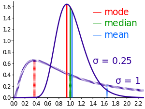
Comparison of the arithmetic mean, median and mode of two skewed (log-normal) distributions.

Geometric visualisation of the mode, median and mean of an arbitrary probability density function.^[5]

In descriptive statistics, the mean may be confused with the median, mode or mid-range, as any of these may be called an "average" (more formally, a measure of central tendency). The mean of a set of observations is the arithmetic average of the values; however, for skewed distributions, the mean is not necessarily the same as the middle value (median), or the most likely value (mode). For example, mean income is typically skewed upwards by a small number of people with very large incomes, so that the majority have an income lower than the mean. By contrast, the median income is the level at which half the population is below and half is above. The mode income is the most likely income, and favors the larger number of people with lower incomes. While the median and mode are often more intuitive measures for such skewed data, many skewed distributions are in fact best described by their mean, including the exponential and Poisson distributions.

Mean of a probability distribution

Main article: Expected value

The mean of a probability distribution is the long-run arithmetic average value of a random variable having that distribution. In this context, it is also known as the expected value. For a discrete probability distribution, the mean is given by $\textstyle \sum xP(x)$ , where the sum is taken over all possible values of the random variable and $P(x)$ is the probability mass function. For a continuous distribution,the mean is $\textstyle \int _{-\infty }^{\infty }xf(x)\,dx$ , where $f(x)$ is the probability density function. In all cases, including those in which the distribution is neither discrete nor continuous, the mean is the Lebesgue integral of the random variable with respect to its probability measure. The mean need not exist or be finite; for some probability distributions the mean is infinite ( $+ \infty$ or $- \infty$ ), while others have no mean.

Generalized means

Power mean

The generalized mean, also known as the power mean or Hölder mean, is an abstraction of the quadratic, arithmetic, geometric and harmonic means. It is defined for a set of n positive numbers x_i by

{\bar {x}}(m)=\left({\frac {1}{n}}\cdot \sum _{i=1}^{n}{x_{i}^{m}}\right)^{\tfrac {1}{m}}

By choosing different values for the parameter m, the following types of means are obtained:

$m\rightarrow \infty$	maximum of $x_{i}$
$m=2$	quadratic mean
$m=1$	arithmetic mean
$m\rightarrow 0$	geometric mean
$m=-1$	harmonic mean
$m\rightarrow -\infty$	minimum of $x_{i}$

ƒ-mean

This can be generalized further as the generalized f-mean

{\bar {x}}=f^{{-1}}\left({{\frac {1}{n}}\cdot \sum _{{i=1}}^{n}{f(x_{i})}}\right)

and again a suitable choice of an invertible ƒ will give

$f(x)=x$	arithmetic mean,
$f(x)={\frac {1}{x}}$	harmonic mean,
$f(x)=x^{m}$	power mean,
$f(x)=\ln x$	geometric mean.

Weighted arithmetic mean

The weighted arithmetic mean (or weighted average) is used if one wants to combine average values from samples of the same population with different sample sizes:

{\bar {x}}={\frac {\sum _{{i=1}}^{n}{w_{i}\cdot x_{i}}}{\sum _{{i=1}}^{n}{w_{i}}}}.

The weights $w_{i}$ represent the sizes of the different samples. In other applications they represent a measure for the reliability of the influence upon the mean by the respective values.

Truncated mean

Sometimes a set of numbers might contain outliers, i.e., data values which are much lower or much higher than the others. Often, outliers are erroneous data caused by artifacts. In this case, one can use a truncated mean. It involves discarding given parts of the data at the top or the bottom end, typically an equal amount at each end, and then taking the arithmetic mean of the remaining data. The number of values removed is indicated as a percentage of total number of values.

Interquartile mean

The interquartile mean is a specific example of a truncated mean. It is simply the arithmetic mean after removing the lowest and the highest quarter of values.

{\bar {x}}={2 \over n}\sum _{{i=(n/4)+1}}^{{3n/4}}{x_{i}}

assuming the values have been ordered, so is simply a specific example of a weighted mean for a specific set of weights.

Mean of a function

Main article: Mean of a function

In some circumstances mathematicians may calculate a mean of an infinite (even an uncountable) set of values. This can happen when calculating the mean value $y_{{{\text{ave}}}}$ of a function $f(x)$ . Intuitively this can be thought of as calculating the area under a section of a curve and then dividing by the length of that section. This can be done crudely by counting squares on graph paper or more precisely by integration. The integration formula is written as:

y_{{{\text{ave}}}}(a,b)={\frac {\int \limits _{{a}}^{{b}}\!f(x)\,dx\,}{b-a}}

Care must be taken to make sure that the integral converges. But the mean may be finite even if the function itself tends to infinity at some points.

Mean of angles and cyclical quantities

Angles, times of day, and other cyclical quantities require modular arithmetic to add and otherwise combine numbers. In all these situations, there will not be a unique mean. For example, the times an hour before and after midnight are equidistant to both midnight and noon. It is also possible that no mean exists. Consider a color wheel -- there is no mean to the set of all colors. In these situations, you must decide which mean is most useful. You can do this by adjusting the values before averaging, or by using a specialized approach for the mean of circular quantities.

Fréchet mean

The Fréchet mean gives a manner for determining the "center" of a mass distribution on a surface or, more generally, Riemannian manifold. Unlike many other means, the Fréchet mean is defined on a space whose elements cannot necessarily be added together or multiplied by scalars. It is sometimes also known as the Karcher mean (named after Hermann Karcher).

Other means

Distribution of the sample mean

Main article: Standard error of the mean

The arithmetic mean of a population, or population mean, is denoted μ. The sample mean (the arithmetic mean of a sample of values drawn from the population) makes a good estimator of the population mean, as its expected value is equal to the population mean (that is, it is an unbiased estimator). The sample mean is a random variable, not a constant, since its calculated value will randomly differ depending on which members of the population are sampled, and consequently it will have its own distribution. For a random sample of n observations from a normally distributed population, the sample mean distribution is normally distributed with mean and variance as follows:

{\bar {x}}\thicksim N\left\{\mu ,{\frac {\sigma ^{2}}{n}}\right\}.

Often, since the population variance is an unknown parameter, it is estimated by the mean sum of squares; when this estimated value is used, the distribution of the sample mean is no longer a normal distribution but rather a Student's t distribution with n − 1 degrees of freedom.

References

↑ Feller, William (1950). Introduction to Probability Theory and its Applications, Vol I. Wiley. p. 221. ISBN 0471257087.
↑ Elementary Statistics by Robert R. Johnson and Patricia J. Kuby, p. 279
↑ Underhill, L.G.; Bradfield d. (1998) Introstat, Juta and Company Ltd. ISBN 0-7021-3838-X p. 181
↑ Schaum's Outline of Theory and Problems of Probability by Seymour Lipschutz and Marc Lipson, p. 141
↑ "AP Statistics Review - Density Curves and the Normal Distributions". Retrieved 16 March 2015.

External links

Weisstein, Eric W. "Mean". MathWorld.

Weisstein, Eric W. "Arithmetic Mean". MathWorld.

Statistics

Descriptive statistics

Continuous data

Center	Mean arithmetic geometric harmonic Median Mode

Dispersion	Variance Standard deviation Coefficient of variation Percentile Range Interquartile range

Shape	Moments Skewness Kurtosis L-moments

Count data

Index of dispersion

Summary tables

Dependence

Graphics

Data collection

Study design	Population Statistic Effect size Statistical power Sample size determination Missing data

Survey methodology	Sampling Standard error stratified cluster Opinion poll Questionnaire

Controlled experiments	Design control optimal Controlled trial Randomized Random assignment Replication Blocking Interaction Factorial experiment

Uncontrolled studies	Observational study Natural experiment Quasi-experiment

Statistical inference

Statistical theory

Frequentist inference

Point estimation	Estimating equations Maximum likelihood Method of moments M-estimator Minimum distance Unbiased estimators Mean-unbiased minimum-variance Rao–Blackwellization Lehmann–Scheffé theorem Median unbiased Plug-in

Interval estimation	Confidence interval Pivot Likelihood interval Prediction interval Tolerance interval Resampling Bootstrap Jackknife

Testing hypotheses	1- & 2-tails Power Uniformly most powerful test Permutation test Randomization test Multiple comparisons

Parametric tests	Likelihood-ratio Wald Score

Specific tests

Z (normal) Student's t-test F

Goodness of fit	Chi-squared Kolmogorov–Smirnov Anderson–Darling Normality (Shapiro–Wilk) Likelihood-ratio test Model selection Cross validation AIC BIC

Rank statistics	Sign Sample median Signed rank (Wilcoxon) Hodges–Lehmann estimator Rank sum (Mann–Whitney) Nonparametric anova 1-way (Kruskal–Wallis) 2-way (Friedman) Ordered alternative (Jonckheere–Terpstra)

Bayesian inference

Correlation	Pearson product–moment Partial correlation Confounding variable Coefficient of determination

Regression analysis	Errors and residuals Regression model validation Mixed effects models Simultaneous equations models Multivariate adaptive regression splines (MARS)

Linear regression	Simple linear regression Ordinary least squares General linear model Bayesian regression

Non-standard predictors	Nonlinear regression Nonparametric Semiparametric Isotonic Robust Heteroscedasticity Homoscedasticity

Generalized linear model	Exponential families Logistic (Bernoulli) / Binomial / Poisson regressions

Partition of variance	Analysis of variance (ANOVA, anova) Analysis of covariance Multivariate ANOVA Degrees of freedom

Categorical / Multivariate / Time-series / Survival analysis

Categorical

Multivariate

Time-series

General	Decomposition Trend Stationarity Seasonal adjustment Exponential smoothing Cointegration Structural break Granger causality

Specific tests	Dickey–Fuller Johansen Q-statistic (Ljung–Box) Durbin–Watson Breusch–Godfrey

Time domain	Autocorrelation (ACF) partial (PACF) Cross-correlation (XCF) ARMA model ARIMA model (Box–Jenkins) Autoregressive conditional heteroskedasticity (ARCH) Vector autoregression (VAR)

Frequency domain	Spectral density estimation Fourier analysis Wavelet

Survival

Survival function	Kaplan–Meier estimator (product limit) Proportional hazards models Accelerated failure time (AFT) model First hitting time

Hazard function	Nelson–Aalen estimator

Test	Log-rank test

Applications

Biostatistics	Bioinformatics Clinical trials / studies Epidemiology Medical statistics

Engineering statistics	Chemometrics Methods engineering Probabilistic design Process / quality control Reliability System identification

Social statistics	Actuarial science Census Crime statistics Demography Econometrics National accounts Official statistics Population statistics Psychometrics

Spatial statistics	Cartography Environmental statistics Geographic information system Geostatistics Kriging

Category
Portal
Commons
WikiProject

This article is issued from Wikipedia - version of the 11/30/2016. The text is available under the Creative Commons Attribution/Share Alike but additional terms may apply for the media files.