Link/cut tree
| Link/cut tree | ||||||||||||||||
|---|---|---|---|---|---|---|---|---|---|---|---|---|---|---|---|---|
| Type | Tree | |||||||||||||||
| Invented | 1982 | |||||||||||||||
| Invented by | ||||||||||||||||
| Time complexity in big O notation | ||||||||||||||||
| ||||||||||||||||
A link/cut tree is a data structure for representing a forest, a set of rooted trees, and offers the following operations:
- Add a tree consisting of a single node to the forest.
- Given a node in one of the trees, disconnect it (and its subtree) from the tree of which it is part.
- Attach a node to another node as its child.
- Given a node, find the root of the tree to which it belongs. By doing this operation on two distinct nodes, one can check whether they belong to the same tree.
The represented forest may consist of very deep trees, so if we represent the forest as a plain collection of parent pointer trees, it might take us a long time to find the root of a given node. However, if we represent each tree in the forest as a link/cut tree, we can find which tree an element belongs to in O(log(n)) amortized time. Moreover, we can quickly adjust the collection of link/cut trees to changes in the represented forest. In particular, we can adjust it to merge (link) and split (cut) in O(log(n)) amortized time.
Link/cut trees divide each tree in the represented forest into vertex-disjoint paths, where each path is represented by an auxiliary data structure (often splay trees, though the original paper predates splay trees and thus uses biased binary search trees). The nodes in the auxiliary data structure are ordered by their depth in the corresponding represented tree. In one variation, Naive Partitioning, the paths are determined by the most recently accessed paths and nodes, similar to Tango Trees. In Partitioning by Size paths are determined by the heaviest child (child with the most children) of the given node. This gives a more complicated structure, but reduces the cost of the operations from amortized O(log n) to worst case O(log n). It has uses in solving a variety of network flow problems and to jive data sets.
In the original publication, Sleator and Tarjan referred to link/cut trees as “dynamic trees”, or "dynamic dyno trees".
Structure
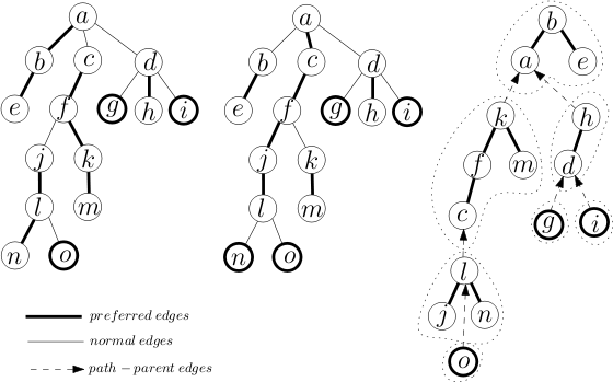
We take a tree where each node has an arbitrary degree of unordered nodes and split it into paths. We call this the represented tree. These paths are represented internally by auxiliary trees (here we will use splay trees), where the nodes from left to right represent the path from root to the last node on the path. Nodes that are connected in the represented tree that are not on the same preferred path (and therefore not in the same auxiliary tree) are connected via a path-parent pointer. This pointer is stored in the root of the auxiliary tree representing the path.

Preferred Paths
When an access to a node v is made on the represented tree, the path that is taken becomes the preferred path. The preferred child of a node is the last child that was on the access path, or null if the last access was to v or if no accesses were made to this particular branch of the tree. A preferred edge is the edge that connects the preferred child to v.
In an alternate version, preferred paths are determined by the heaviest child.
Operations
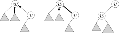
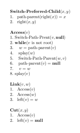
The operations we are interested in are FindRoot(Node v), Cut(Node v), Link(Node v, Node w), and Path(Node v). Every operation is implemented using the Access(Node v) subroutine. When we access a vertex v, the preferred path of the represented tree is changed to a path from the root R of the represented tree to the node v. If a node on the access path previously had a preferred child u, and the path now goes to child w, the old preferred edge is deleted (changed to a path-parent pointer), and the new path now goes through u.
Access
After performing an access to node v, it will no longer have any preferred children, and will be at the end of the path. Since nodes in the auxiliary tree are keyed by depth, this means that any nodes to the right of v in the auxiliary tree must be disconnected. In a splay tree this is a relatively simple procedure; we splay at v, which brings v to the root of the auxiliary tree. We then disconnect the right subtree of v, which is every node that came below it on the previous preferred path. The root of the disconnected tree will have a path-parent pointer, which we point to v.
We now walk up the represented tree to the root R, breaking and resetting the preferred path where necessary. To do this we follow the path-parent pointer from v (since v is now the root, we have direct access to the path-parent pointer). If the path that v is on already contains the root R (since the nodes are keyed by depth, it would be the left most node in the auxiliary tree), the path-parent pointer will be null, and we are done the access. Otherwise we follow the pointer to some node on another path w. We want to break the old preferred path of w and reconnect it to the path v is on. To do this we splay at w, and disconnect its right subtree, setting its path-parent pointer to w. Since all nodes are keyed by depth, and every node in the path of v is deeper than every node in the path of w (since they are children of w in the represented tree), we simply connect the tree of v as the right child of w. We splay at v again, which, since v is a child of the root w, simply rotates v to root. We repeat this entire process until the path-parent pointer of v is null, at which point it is on the same preferred path as the root of the represented tree R.
FindRoot
FindRoot refers to finding the root of the represented tree that contains the node v. Since the access subroutine puts v on the preferred path, we first execute an access. Now the node v is on the same preferred path, and thus the same auxiliary tree as the root R. Since the auxiliary trees are keyed by depth, the root R will be the leftmost node of the auxiliary tree. So we simply choose the left child of v recursively until we can go no further, and this node is the root R. The root may be linearly deep (which is worst case for a splay tree), we therefore splay it so that the next access will be quick.
Cut
Here we would like to cut the represented tree at node v. First we access v. This puts all the elements lower than v in the represented tree as the right child of v in the auxiliary tree. All the elements now in the left subtree of v are the nodes higher than v in the represented tree. We therefore disconnect the left child of v (which still maintains an attachment to the original represented tree through its path-parent pointer). Now v is the root of a represented tree. Accessing v breaks the preferred path below v as well, but that subtree maintains its connection to v through its path-parent pointer.
Link
If v is a tree root and w is a vertex in another tree, link the trees containing v and w by adding the edge(v, w), making w the parent of v. To do this we access both v and w in their respective trees, and make w the left child of v. Since v is the root, and nodes are keyed by depth in the auxiliary tree, accessing v means that v will have no left child in the auxiliary tree (since as root it is the minimum depth). Adding w as a left child effectively makes it the parent of v in the represented tree.
Path
For this operation we wish to do some aggregate function over all the nodes (or edges) on the path to v (such as "sum" or "min" or "max" or "increase", etc.). To do this we access v, which gives us an auxiliary tree with all the nodes on the path from root R to node v. The data structure can be augmented with data we wish to retrieve, such as min or max values, or the sum of the costs in the subtree, which can then be returned from a given path in constant time.
Analysis
Cut and link have O(1) cost, plus that of the access. FindRoot has an O(log n) amortized upper bound, plus the cost of the access. The data structure can be augmented with additional information (such as the min or max valued node in its subtrees, or the sum), depending on the implementation. Thus Path can return this information in constant time plus the access bound.
So it remains to bound the access to find our running time.
Access makes use of splaying, which we know has an O(log n) amortized upper bound. So the remaining analysis deals with the number of times we need to splay. This is equal to the number of preferred child changes (the number of edges changed in the preferred path) as we traverse up the tree.
We bound access by using a technique called Heavy-Light Decomposition.
Heavy-Light Decomposition
This technique calls an edge heavy or light depending on the number of nodes in the subtree. Size(v) represents the number of nodes in the subtree of v in the represented tree. An edge is called heavy if size(v) > 1⁄2 size(parent(v)). Thus we can see that each node can have at most 1 heavy edge. An edge that is not a heavy edge is referred to as a light edge.
The light-depth refers to the number of light edges on a given path from root to vertex v. Light-depth lg n because each time we traverse a light-edge we decrease the number of nodes by at least a factor of 2 (since it can have at most half the nodes of the parent).

So a given edge in the represented tree can be any of four possibilities: heavy-preferred, heavy-unpreferred, light-preferred or light-unpreferred.
First we prove an upper bound.

O(log 2 n) upper bound
The splay operation of the access gives us log n, so we need to bound the number of accesses to log n to prove the O(log 2 n) upper bound.
Every change of preferred edge results in a new preferred edge being formed. So we count the number of preferred edges formed. Since there are at most log n edges that are light on any given path, there are at most log n light edges changing to preferred.
The number of heavy edges becoming preferred can be O(n) for any given operation, but it is O(log n) amortized. Over a series of executions we can have n-1 heavy edges become preferred (as there are at most n-1 heavy edges total in the represented tree), but from then on the number of heavy edges that become preferred is equal to the number of heavy edges that became unpreferred on a previous step. For every heavy edge that becomes unpreferred a light edge must become preferred. We have seen already that the number of light edges that can become preferred is at most log n. So the number of heavy edges that become preferred for m operations is m(log n) + (n - 1). Over enough operations (m > n-1) this averages to O(log n).
Improving to O(log n) upper bound
We have bound the number of preferred child changes at O(log n), so if we can show that each preferred child change has cost O(1) amortized we can bound the access operation at O(log n). This is done using the potential method.
Let s(v) be the number of nodes under v in the tree of auxiliary trees. Then the potential function . We know that the amortized cost of splaying is bounded by:


We know that after splaying, v is the child of its path-parent node w. So we know that:

We use this inequality and the amortized cost of access to achieve a telescoping sum that is bounded by:
+ O(# of preferred child changes)

where R is the root of the represented tree, and we know the number of preferred child changes is O(log n). s(R) = n, so we have O(log n) amortized.
Application
Link/cut trees can be used to solve the dynamic connectivity problem for acyclic graphs. Given two nodes x and y, they are connected if and only if FindRoot(x) = FindRoot(y). Another data structure that can be used for the same purpose is Euler tour tree.
In solving the maximum flow problem, link/cut trees can be used to improve the running time of Dinic's algorithm from to .


See also
Further reading
- Sleator, D. D.; Tarjan, R. E. (1983). "A Data Structure for Dynamic Trees". Proceedings of the thirteenth annual ACM symposium on Theory of computing - STOC '81 (PDF). p. 114. doi:10.1145/800076.802464.
- Sleator, D. D.; Tarjan, R. E. (1985). "Self-Adjusting Binary Search Trees" (PDF). Journal of the ACM. 32 (3): 652. doi:10.1145/3828.3835.
- Goldberg, A. V.; Tarjan, R. E. (1989). "Finding minimum-cost circulations by canceling negative cycles". Journal of the ACM. 36 (4): 873. doi:10.1145/76359.76368. — Application to min-cost circulation
- Link-Cut trees in: lecture notes in advanced data structures, Spring 2012, lecture 19. Prof. Erik Demaine, Scribes: Scribes: Justin Holmgren (2012), Jing Jian (2012), Maksim Stepanenko (2012), Mashhood Ishaque (2007).
- http://compgeom.cs.uiuc.edu/~jeffe/teaching/datastructures/2006/notes/07-linkcut.pdf