Leading-order term
The leading-order terms (or corrections) within a mathematical equation, expression or model are the terms with the largest order of magnitude.[1][2] The sizes of the different terms in the equation(s) will change as the variables change, and hence, which terms are leading-order may also change.
A common and powerful way of simplifying and understanding a wide variety of complicated mathematical models is to investigate which terms are the largest (and therefore most important), for particular sizes of the variables and parameters, and analyse the behaviour produced by just these terms (regarding the other smaller terms as negligible).[3][4] This gives the main behaviour - the true behaviour is only small deviations away from this. This main behaviour may be captured sufficiently well by just the strictly leading-order terms, or it may be decided that slightly smaller terms should also be included. In which case, the phrase leading-order terms might be used informally to mean this whole group of terms. The behaviour produced by just the group of leading-order terms is called the leading-order behaviour of the model.
Basic example
|| Leading-order terms highlighted in pink.
| x | 0.001 | 0.1 | 0.5 | 2 | 10 |
|---|---|---|---|---|---|
| x3 | 0.000000001 | 0.001 | 0.125 | 8 | 1000 |
| 5x | 0.005 | 0.5 | 2.5 | 10 | 50 |
| 0.1 | 0.1 | 0.1 | 0.1 | 0.1 | 0.1 |
| y | 0.105000001 | 0.601 | 2.725 | 18.1 | 1050.1 |
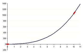
Consider the equation y=x3+5x+0.1. For five different values of x, the table shows the sizes of the four terms in this equation, and which ones are leading-order. As x increases further, the leading-order terms stay as x3 and y, but as x decreases and then becomes more and more negative, which terms are leading-order again changes.
There is no strict cut-off for when two terms should or should not be regarded as approximately the same order, or magnitude. One possible rule of thumb is that two terms that are within a factor of 10 (one order of magnitude) of each other should be regarded as of about the same order, and two terms that are not within a factor of 100 (two orders of magnitude) of each other should not. However, in between is a grey area, so there are no fixed boundaries where terms are to be regarded as approximately leading-order and where not. Instead the terms fade in and out, as the variables change. Deciding whether terms in a model are leading-order (or approximately leading-order), and if not, whether they are small enough to be regarded as negligible, (two different questions), is often a matter of investigation and judgement, and will depend on the context.
Leading-order behaviour
Equations with only one leading-order term are possible, but rare. For example, the equation 100 = 1 + 1 + 1 + ... + 1, (where the right hand side comprises one hundred 1's). For any particular combination of values for the variables and parameters, an equation will typically contain at least two leading-order terms, and other lower-order terms. In this case, by making the assumption that the lower-order terms, and the parts of the leading-order terms that are the same size as the lower-order terms (perhaps the second or third significant figure onwards), are negligible, a new equation may be formed by dropping all these lower-order terms and parts of the leading-order terms. The remaining terms provide the leading-order equation, or leading-order balance,[5] or dominant balance,[6][7][8] and creating a new equation just involving these terms is known as taking an equation to leading-order. The solutions to this new equation are called the leading-order solutions[9][10] to the original equation. Analysing the behaviour given by this new equation gives the leading-order behaviour[11][12] of the model for these values of the variables and parameters. The size of the error in making this approximation is normally roughly the size of the largest neglected term.
Suppose we want to understand the leading-order behaviour of the example above.
- When x=0.001, the x3 and 5x terms may be regarded as negligible, and dropped, along with any values in the third decimal places onwards in the two remaining terms. This gives the leading-order balance y=0.1. Thus the leading-order behaviour of this equation at x=0.001 is that y is constant.
- Similarly, when x=10, the 5x and 0.1 terms may be regarded as negligible, and dropped, along with any values in the third significant figure onwards in the two remaining terms. This gives the leading-order balance y=x3. Thus the leading-order behaviour of this equation at x=10 is that y increases cubically with x.
The main behaviour of y may thus be investigated at any value of x. The leading-order behaviour is more complicated when more terms are leading-order. At x=2 there is a leading-order balance between the cubic and linear dependencies of y on x.
Note that this description of finding leading-order balances and behaviours gives only an outline description of the process - it is not mathematically rigorous.
Next-to-leading order
Of course, y is not actually completely constant at x=0.001 - this is just its main behaviour in the vicinity of this point. It may be that retaining only the leading-order (or approximately leading-order) terms, and regarding all the other smaller terms as negligible, is insufficient (when using the model for future prediction, for example), and so it may be necessary to also retain the set of next largest terms. These can be called the next-to-leading order (NLO) terms or corrections.[13][14] The next set of terms down after that can be called the next-to-next-to-leading order (NNLO) terms or corrections.[15]
Usage
Matched asymptotic expansions
Leading-order simplification techniques are used in conjunction with the method of matched asymptotic expansions, when the accurate approximate solution in each subdomain is the leading-order solution.[3][16][17]
Simplifying the Navier-Stokes equations
For particular fluid flow scenarios, the (very general) Navier–Stokes equations may be considerably simplified by considering only the leading-order components. For example, the Stokes flow equations.[18] Also, the thin film equations of lubrication theory.
References
- ↑ J.K.Hunter, Asymptotic Analysis and Singular Perturbation Theory, 2004. http://www.math.ucdavis.edu/~hunter/notes/asy.pdf
- ↑ NYU course notes
- 1 2 Mitchell, M. J.; et al. (2010). "A model of carbon dioxide dissolution and mineral carbonation kinetics". Proceedings of the Royal Society A. 466 (2117): 1265–1290. doi:10.1098/rspa.2009.0349.
- ↑ Woollard, H. F.; et al. (2008). "A multi-scale model for solute transport in a wavy-walled channel" (PDF). Journal of Engineering Mathematics. 64: 25–48. doi:10.1007/s10665-008-9239-x.
- ↑ Sternberg, P.; Bernoff, A. J. (1998). "Onset of Superconductivity in Decreasing Fields for General Domains". Journal of Mathematical Physics. 39 (3): 1272–1284. doi:10.1063/1.532379.
- ↑ Salamon, T.R.; et al. (1995). "The role of surface tension in the dominant balance in the die swell singularity". Physics of Fluids. 7 (10): 2328. doi:10.1063/1.868746.
- ↑ Gorshkov, A. V.; et al. (2008). "Coherent Quantum Optical Control with Subwavelength Resolution". Physical Review Letters. 100 (9): 93005. arXiv:0706.3879
 . Bibcode:2008PhRvL.100i3005G. doi:10.1103/PhysRevLett.100.093005.
 - ↑ Lindenberg, K.; et al. (1994). "Diffusion-Limited Binary Reactions: The Hierarchy of Nonclassical Regimes for Correlated Initial Conditions" (PDF). Journal of Physical Chemistry. 98 (13): 3389–3397. doi:10.1021/j100064a020.
- ↑ Żenczykowski, P. (1988). "Kobayashi-Maskawa matrix from the leading-order solution of the n-generation Fritzsch model". Physical Review D. 38 (1): 332–336. doi:10.1103/PhysRevD.38.332.
- ↑ Horowitz, G. T.; Tseytlin, A. A. (1994). "Extremal black holes as exact string solutions". Physical Review Letters. 73 (25): 3351–3354. arXiv:hep-th/9408040. doi:10.1103/PhysRevLett.73.3351. PMID 10057359.
- ↑ Hüseyin, A. (1980). "The leading-order behaviour of the two-photon scattering amplitudes in QCD". Nuclear Physics B. 163: 453–460. doi:10.1016/0550-3213(80)90411-3.
- ↑ Kruczenski, M.; Oxman, L.E.; Zaldarriaga, M. (1999). "Large squeezing behaviour of cosmological entropy generation". Classical and Quantum Gravity. 11 (9): 2317–2329. arXiv:gr-qc/9403024. doi:10.1088/0264-9381/11/9/013.
- ↑ Campbell, J.; Ellis, R.K. (2002). "Next-to-leading order corrections to W + 2 jet and Z + 2 jet production at hadron colliders". Physical Review D. 65 (11): 113007. arXiv:hep-ph/0202176. doi:10.1103/PhysRevD.65.113007.
- ↑ Catani, S.; Seymour, M.H. (1996). "The Dipole Formalism for the Calculation of QCD Jet Cross Sections at Next-to-Leading Order". Physics Letters B. 378 (1): 287–301. arXiv:hep-ph/9602277. doi:10.1016/0370-2693(96)00425-X.
- ↑ Kidonakis, N.; Vogt, R. (2003). "Next-to-next-to-leading order soft-gluon corrections in top quark hadroproduction". Physical Review D. 68 (11): 114014. arXiv:hep-ph/0308222. doi:10.1103/PhysRevD.68.114014.
- ↑ Rubinstein, B.Y.; Pismen, L.M. (1994). "Vortex motion in the spatially inhomogeneous conservative Ginzburg-Landau model" (PDF). Physica D: Nonlinear Phenomena. 78 (1): 1–10. doi:10.1016/0167-2789(94)00119-7.
- ↑ Kivshar, Y.S.; et al. (1998). "Dynamics of optical vortex solitons" (PDF). Optics Communications. 152 (1): 198–206. Bibcode:1998OptCo.152..198K. doi:10.1016/S0030-4018(98)00149-7.
- ↑ Cornell University notes