Rotation matrix

In linear algebra, a rotation matrix is a matrix that is used to perform a rotation in Euclidean space. For example the matrix

R={\begin{bmatrix}\cos \theta &-\sin \theta \\\sin \theta &\cos \theta \\\end{bmatrix}}

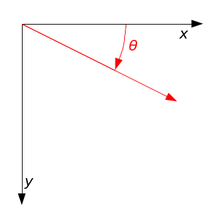
rotates points in the xy-Cartesian plane counter-clockwise through an angle $θ$ about the origin of the Cartesian coordinate system. To perform the rotation using a rotation matrix $R$ , the position of each point must be represented by a column vector v, containing the coordinates of the point. A rotated vector is obtained by using the matrix multiplication $R$ v.

Rotation matrices also provide a means of numerically representing an arbitrary rotation of the axes about the origin, without appealing to angular specification. These coordinate rotations are a natural way to express the orientation of a camera, or the attitude of a spacecraft, relative to a reference axes-set. Once an observational platform's local X-Y-Z axes are expressed numerically as three direction vectors in world coordinates, they together comprise the columns of the rotation matrix $R$ (world → platform) that transforms directions (expressed in world coordinates) into equivalent directions expressed in platform-local coordinates.

The examples in this article apply to active rotations of vectors counter-clockwise in a right-handed coordinate system by pre-multiplication. If any one of these is changed (e.g. rotating axes instead of vectors, i.e. a passive transformation), then the inverse of the example matrix should be used, which coincides precisely with its transpose.

Since matrix multiplication has no effect on the zero vector (the coordinates of the origin), rotation matrices can only be used to describe rotations about the origin of the coordinate system. Rotation matrices provide an algebraic description of such rotations, and are used extensively for computations in geometry, physics, and computer graphics.

Rotation matrices are square matrices, with real entries. More specifically, they can be characterized as orthogonal matrices with determinant 1; that is, a square matrix $R$ is a rotation matrix if $R T = R -1$ and $det R = 1$ .

In some literature, the term rotation is generalized to include improper rotations, characterized by orthogonal matrices with determinant −1 (instead of +1). These combine proper rotations with reflections (which invert orientation). In other cases, where reflections are not being considered, the label proper may be dropped. This convention is followed in this article.

The set of all orthogonal matrices of size $n$ with determinant +1 forms a group known as the special orthogonal group $SO(n)$ . The most important special case is that of the rotation group SO(3). The set of all orthogonal matrices of size $n$ with determinant +1 or -1 forms the (general) orthogonal group $O(n)$ .

In two dimensions

A counterclockwise rotation of a vector through angle

θ

. The vector is initially aligned with the

x

-axis.

In two dimensions, every rotation matrix has the following form,

R(\theta )={\begin{bmatrix}\cos \theta &-\sin \theta \\\sin \theta &\cos \theta \\\end{bmatrix}}

This rotates column vectors by means of the following matrix multiplication,

{\begin{bmatrix}x'\\y'\\\end{bmatrix}}={\begin{bmatrix}\cos \theta &-\sin \theta \\\sin \theta &\cos \theta \\\end{bmatrix}}{\begin{bmatrix}x\\y\\\end{bmatrix}}

So the coordinates (x',y') of the point (x,y) after rotation are

x'=x\cos \theta -y\sin \theta \,

y'=x\sin \theta +y\cos \theta \,

The direction of vector rotation is counterclockwise if $θ$ is positive (e.g. 90°), and clockwise if $θ$ is negative (e.g. −90°). Thus the clockwise rotation matrix is found as

R(-\theta )={\begin{bmatrix}\cos \theta &\sin \theta \\-\sin \theta &\cos \theta \\\end{bmatrix}}\,

Note that the two-dimensional case is the only non-trivial (i.e. not $1$ -dimensional) case where the rotation matrices group is commutative, so that it does not matter in which order multiple rotations are performed. An alternative convention uses rotating axes,^[1] and the above matrices also represent a rotation of the axes clockwise through an angle $θ$ .

Non-standard orientation of the coordinate system

A rotation through angle

θ

with non-standard axes.

If a standard right-handed Cartesian coordinate system is used, with the $x$ -axis to the right and the $y$ -axis up, the rotation $R (θ)$ is counterclockwise. If a left-handed Cartesian coordinate system is used, with $x$ directed to the right but $y$ directed down, $R (θ)$ is clockwise. Such non-standard orientations are rarely used in mathematics but are common in 2D computer graphics, which often have the origin in the top left corner and the $y$ -axis down the screen or page.^[2]

See below for other alternative conventions which may change the sense of the rotation produced by a rotation matrix.

Common rotations

Particularly useful are the matrices for 90°, 180°, and 270° rotations, ${\begin{aligned}R(90^{\circ })&={\begin{bmatrix}0&-1\\[3pt]1&0\\\end{bmatrix}}\qquad &{\text{(90° counter-clockwise rotation)}},\\R(180^{\circ })&={\begin{bmatrix}-1&0\\[3pt]0&-1\\\end{bmatrix}}\qquad &{\text{(180° rotation in either direction – a half-turn)}},\\R(270^{\circ })&={\begin{bmatrix}0&1\\[3pt]-1&0\\\end{bmatrix}}\qquad &{\text{(270° counter-clockwise rotation, the same as a 90° clockwise rotation)}}.\end{aligned}}$

In three dimensions

Basic rotations

A basic rotation (also called elemental rotation) is a rotation about one of the axes of a Coordinate system. The following three basic rotation matrices rotate vectors by an angle θ about the x, y, or z axis, in three dimensions, using the right-hand rule—which codifies their alternating signs. (The same matrices can also represent a clockwise rotation of the axes.^{[nb 1]})

{\begin{alignedat}{1}R_{x}(\theta )&={\begin{bmatrix}1&0&0\\0&\cos \theta &-\sin \theta \\[3pt]0&\sin \theta &\cos \theta \\[3pt]\end{bmatrix}}\\[6pt]R_{y}(\theta )&={\begin{bmatrix}\cos \theta &0&\sin \theta \\[3pt]0&1&0\\[3pt]-\sin \theta &0&\cos \theta \\\end{bmatrix}}\\[6pt]R_{z}(\theta )&={\begin{bmatrix}\cos \theta &-\sin \theta &0\\[3pt]\sin \theta &\cos \theta &0\\[3pt]0&0&1\\\end{bmatrix}}\end{alignedat}}

For column vectors, each of these basic vector rotations appears counter-clockwise when the axis about which they occur points toward the observer, the coordinate system is right-handed, and the angle $θ$ is positive. $R z$ , for instance, would rotate toward the $y$ -axis a vector aligned with the $x$ -axis, as can easily be checked by operating with $R z$ on the vector $(1,0,0)$ :

R_{z}(90^{\circ }){\begin{bmatrix}1\\0\\0\\\end{bmatrix}}={\begin{bmatrix}\cos 90^{\circ }&-\sin 90^{\circ }&0\\\sin 90^{\circ }&\quad \cos 90^{\circ }&0\\0&0&1\\\end{bmatrix}}{\begin{bmatrix}1\\0\\0\\\end{bmatrix}}={\begin{bmatrix}0&-1&0\\1&0&0\\0&0&1\\\end{bmatrix}}{\begin{bmatrix}1\\0\\0\\\end{bmatrix}}={\begin{bmatrix}0\\1\\0\\\end{bmatrix}}

This is similar to the rotation produced by the above mentioned $2$ -D rotation matrix. See below for alternative conventions which may apparently or actually invert the sense of the rotation produced by these matrices.

General rotations

Other rotation matrices can be obtained from these three using matrix multiplication. For example, the product

R=R_{z}(\alpha )\,R_{y}(\beta )\,R_{x}(\gamma )\,\!

represents a rotation whose yaw, pitch, and roll angles are $α, β$ and $γ$ , respectively. More formally, it is an intrinsic rotation whose Tait-Bryan angles are $α, β, γ$ , about axes $z, y, x$ respectively. Similarly, the product

R=R_{z}(\gamma )\,R_{y}(\beta )\,R_{x}(\alpha )\,\!

represents an extrinsic rotation whose (improper) Euler angles are $α, β, γ$ about axes $x, y, z$ .

These matrices produce the desired effect only if they are used to pre-multiply column vectors (see Ambiguities for more details).

Conversion from and to axis-angle

Every rotation in three dimensions is defined by its axis — a direction that is left fixed by the rotation — and its angle — the amount of rotation about that axis (Euler rotation theorem).

There are several methods to compute an axis and an angle from a rotation matrix (see also axis-angle). Here, we only describe the method based on the computation of the eigenvectors and eigenvalues of the rotation matrix. It is also possible to use the trace of the rotation matrix.

Determining the axis

A rotation R around axis u can be decomposed using 3 endomorphisms P, (I − P), and Q (click to enlarge).

Given a $3 \times 3$ rotation matrix $R$ , a vector $u$ parallel to the rotation axis must satisfy

R{\textbf {u}}={\textbf {u}}~,

since the rotation of $u$ around the rotation axis must result in $u$ . The equation above may be solved for $u$ which is unique up to a scalar factor unless $R = I$ .

Further, the equation may be rewritten

R{\textbf {u}}=I{\textbf {u}}\quad \Rightarrow \quad (R-I){\textbf {u}}=0~,

which shows that $u$ lies in the null space of $R - I$ .

Viewed in another way, $u$ is an eigenvector of $R$ corresponding to the eigenvalue $λ = 1$ . Every rotation matrix must have this eigenvalue, the other two eigenvalues being complex conjugates of each other. It follows that a general rotation matrix in three dimensions has, up to a multiplicative constant, only one real eigenvector.

One way to determine the rotation axis is by showing that:

$0=R^{T}0+0$ $=R^{T}(R-I)\mathbf {u} +(R-I)\mathbf {u}$ $=(R^{T}R-R^{T}+R-I)\mathbf {u}$ $=(I-R^{T}+R-I)\mathbf {u}$ $=(R-R^{T})\mathbf {u} ~$

Since $(R-R^{T})$ is a skew-symmetric matrix, we can choose $u$ such that $[\mathbf {u} ]_{\times }=(R-R^{T})$ . Matrix-vector product becomes a cross product of a vector with itself, ensuring result is zero:

$(R-R^{T})\mathbf {u} =[\mathbf {u} ]_{\times }\mathbf {u} =\mathbf {u} \times \mathbf {u} =0~$

Therefore, if $R={\begin{bmatrix}a&b&c\\d&e&f\\g&h&i\\\end{bmatrix}}$ , then $\mathbf {u} ={\begin{bmatrix}h-f\\c-g\\d-b\\\end{bmatrix}}$ . Magnitude of $u$ computed this way is $\|\mathbf {u} \|=2\sin \theta$ , where $θ$ is the angle of rotation.

Determining the angle

To find the angle of a rotation, once the axis of the rotation is known, select a vector $v$ perpendicular to the axis. Then the angle of the rotation is the angle between $v$ and $R v$ .

A more direct method, however, is to simply calculate the trace, i.e., the sum of the diagonal elements of the rotation matrix. Care should be taken to select the right sign for the angle $θ$ to match the chosen axis:

\operatorname {Tr} (R)=1+2\cos \theta ~.

Rotation matrix from axis and angle

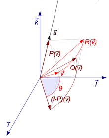
For some applications, it is helpful to be able to make a rotation with a given axis. Given a unit vector u = (u_x, u_y, u_z), where u_x² + u_y² + u_z² = 1, the matrix for a rotation by an angle of θ about an axis in the direction of u is^[3]

R={\begin{bmatrix}\cos \theta +u_{x}^{2}\left(1-\cos \theta \right)&u_{x}u_{y}\left(1-\cos \theta \right)-u_{z}\sin \theta &u_{x}u_{z}\left(1-\cos \theta \right)+u_{y}\sin \theta \\u_{y}u_{x}\left(1-\cos \theta \right)+u_{z}\sin \theta &\cos \theta +u_{y}^{2}\left(1-\cos \theta \right)&u_{y}u_{z}\left(1-\cos \theta \right)-u_{x}\sin \theta \\u_{z}u_{x}\left(1-\cos \theta \right)-u_{y}\sin \theta &u_{z}u_{y}\left(1-\cos \theta \right)+u_{x}\sin \theta &\cos \theta +u_{z}^{2}\left(1-\cos \theta \right)\end{bmatrix}}.

This can be written more concisely as

R=\cos \theta \mathbf {I} +\sin \theta [\mathbf {u} ]_{\times }+(1-\cos \theta )\mathbf {u} \otimes \mathbf {u} ~,

where $[\mathbf {u} ]_{\times }$ is the cross product matrix of u, $\otimes$ is the tensor product and I is the Identity matrix, or alternatively as $R_{jk}={\begin{cases}\cos ^{2}{\frac {\theta }{2}}+\sin ^{2}{\frac {\theta }{2}}\left(2u_{j}^{2}-1\right),\quad &{\text{if }}j=k\\2u_{j}u_{k}\sin ^{2}{\frac {\theta }{2}}+\epsilon _{jkl}u_{l}\sin \theta ,\quad &{\text{if }}j\neq k\end{cases}}$

where $\epsilon_{jkl}$ is the Levi-Civita symbol with $\epsilon _{{123}}=1$ . This is a matrix form of Rodrigues' rotation formula, (or the equivalent, differently parameterized Euler–Rodrigues formula) with^[4]

\mathbf {u} \otimes \mathbf {u} =\mathbf {u} \mathbf {u} ^{T}={\begin{bmatrix}u_{x}^{2}&u_{x}u_{y}&u_{x}u_{z}\\[3pt]u_{x}u_{y}&u_{y}^{2}&u_{y}u_{z}\\[3pt]u_{x}u_{z}&u_{y}u_{z}&u_{z}^{2}\end{bmatrix}},\qquad [\mathbf {u} ]_{\times }={\begin{bmatrix}0&-u_{z}&u_{y}\\[3pt]u_{z}&0&-u_{x}\\[3pt]-u_{y}&u_{x}&0\end{bmatrix}}.

If the 3D space is right-handed, this rotation will be counterclockwise when u points towards the observer (Right-hand rule). Rotations in the counterclockwise (anticlockwise) direction are considered positive rotations.

Note the striking merely apparent differences to the equivalent Lie-algebraic formulation below, #Exponential map.

Properties of a rotation matrix

For any rotation matrix R acting on $ℝ n$ ,

$R^{T}=R^{-1}$ (The rotation is an orthogonal matrix)

It follows that:

$\det R=\pm 1$

A rotation is termed proper if $\det R=1$ and improper if $\det R=-1$ . For even dimensions (n even), the eigenvalues of a rotation matrix occur as pairs of complex conjugates which are roots of unity and may be written $e^{\pm i\theta _{k}}$ . Therefore, there may be no set of vectors which are unaffected by the rotation, and thus no axis of rotation. If there are any real eigenvalues, they will equal unity and will occur in pairs, and the axis of rotation will be an even dimensional subspace of the whole space. For odd dimensions, there will be an odd number of such eigenvalues, with at least one eigenvalue being unity, and the axis of rotation will be an odd dimensional subspace of the whole space.

For example, in 2-space (n=2), there are either two complex eigenvalues or two real eigenvalues equal to unity. In the case of the two unit eigenvalues, the rotation is a null rotation, but otherwise, there is no axis of rotation. In 3-space (n=3), there will be an axis of rotation (a 1-D manifold, or a line through the origin) or the rotation will be null. In 4-space (n=4), there may be no axes of rotation, or there may be a 2 dimensional axis, a plane through the origin, called the "axis plane". As always, when all eigenvalues are unity, the rotation is a null rotation.

The trace of a rotation matrix will be equal to the sum of its eigenvalues. For n=2 the two eigenvalues are $e^{\pm i\theta }$ and the trace will be $2\cos(\theta )$ where $\theta$ is the rotation angle about the origin. For n=3 the three eigenvalues are 1 and $e^{\pm i\theta }$ where $\theta$ is the rotation angle about the axis-line. The trace will be $1+2\cos(\theta )$ . For n=4, the four eigenvalues are of the form $e^{\pm i\theta }$ and $e^{\pm i\phi }$ and the trace will be $2(\cos(\theta )+\cos(\phi ))$ . If one of the angles, say $\theta$ , is equal to zero, then the rotation will be a "simple" rotation, with two unit eigenvalues and the other angle ( $\phi$ ) will be the angle of rotation about the axis-plane spanned by the two eigenvectors with eigenvalues of unity. Otherwise, there will be no axis-plane of rotation. If $\theta =\phi$ (an "isoclinic" rotation), the eigenvalues will be $e^{\pm i\theta }$ repeated twice, and every vector from the origin will be rotated through the angle $\theta$ . The trace will be $4\cos(\theta )$ .

Examples

The 2×2 rotation matrix

Q={\begin{bmatrix}0&1\\-1&0\end{bmatrix}}

corresponds to a 90° planar rotation clockwise about the origin.

The transpose of the 2×2 matrix

M={\begin{bmatrix}0.936&0.352\\0.352&-0.936\end{bmatrix}}

is its inverse, but since its determinant is −1, this is not a rotation matrix; it is a reflection across the line 11y = 2x.

The 3×3 rotation matrix

Q={\begin{bmatrix}1&0&0\\0&{\frac {\sqrt {3}}{2}}&{\frac {1}{2}}\\0&-{\frac {1}{2}}&{\frac {\sqrt {3}}{2}}\end{bmatrix}}

corresponds to a −30° rotation around the x axis in three-dimensional space.

The 3×3 rotation matrix

Q={\begin{bmatrix}0.36&0.48&-0.8\\-0.8&0.60&0\\0.48&0.64&0.60\end{bmatrix}}

corresponds to a rotation of approximately −74° around the axis (−¹⁄₃,²⁄₃,²⁄₃) in three-dimensional space.

The 3×3 permutation matrix

P={\begin{bmatrix}0&0&1\\1&0&0\\0&1&0\end{bmatrix}}

is a rotation matrix, as is the matrix of any even permutation, and rotates through 120° about the axis x = y = z.

The 3×3 matrix

M={\begin{bmatrix}3&-4&1\\5&3&-7\\-9&2&6\end{bmatrix}}

has determinant +1, but is not orthogonal (its transpose is not its inverse), so it is not a rotation matrix.

The 4×3 matrix

M={\begin{bmatrix}0.5&-0.1&0.7\\0.1&0.5&-0.5\\-0.7&0.5&0.5\\-0.5&-0.7&-0.1\end{bmatrix}}

is not square, and so cannot be a rotation matrix; yet M^TM yields a 3×3 identity matrix (the columns are orthonormal).

The 4×4 matrix

Q={\begin{bmatrix}-1&0&0&0\\0&-1&0&0\\0&0&-1&0\\0&0&0&-1\end{bmatrix}}

describes an isoclinic rotation, a rotation through equal angles (180°) through two orthogonal planes.

The 5×5 rotation matrix

Q={\begin{bmatrix}0&-1&0&0&0\\1&0&0&0&0\\0&0&-1&0&0\\0&0&0&-1&0\\0&0&0&0&1\end{bmatrix}}

rotates vectors in the plane of the first two coordinate axes 90°, rotates vectors in the plane of the next two axes 180°, and leaves the last coordinate axis unmoved.

Geometry

In Euclidean geometry, a rotation is an example of an isometry, a transformation that moves points without changing the distances between them. Rotations are distinguished from other isometries by two additional properties: they leave (at least) one point fixed, and they leave "handedness" unchanged. By contrast, a translation moves every point, a reflection exchanges left- and right-handed ordering, and a glide reflection does both.

A rotation that does not leave "handedness" unchanged is an improper rotation or a rotoinversion.

If a fixed point is taken as the origin of a Cartesian coordinate system, then every point can be given coordinates as a displacement from the origin. Thus one may work with the vector space of displacements instead of the points themselves. Now suppose $(p 1,\dots, p n)$ are the coordinates of the vector $p$ from the origin, $O$ , to point $P$ . Choose an orthonormal basis for our coordinates; then the squared distance to $P$ , by Pythagoras, is

d^{2}(O,P)=\|{\mathbf {p}}\|^{2}=\sum _{r=1}^{n}p_{r}^{2}

which can be computed using the matrix multiplication

\|{\mathbf {p}}\|^{2}={\begin{bmatrix}p_{1}\cdots p_{n}\end{bmatrix}}{\begin{bmatrix}p_{1}\\\vdots \\p_{n}\end{bmatrix}}={\mathbf {p}}^{T}{\mathbf {p}}.

A geometric rotation transforms lines to lines, and preserves ratios of distances between points. From these properties it can be shown that a rotation is a linear transformation of the vectors, and thus can be written in matrix form, $Q p$ . The fact that a rotation preserves, not just ratios, but distances themselves, is stated as

{\mathbf {p}}^{T}{\mathbf {p}}=(Q{\mathbf {p}})^{T}(Q{\mathbf {p}}),\,\!

{\begin{aligned}{\mathbf {p}}^{T}I{\mathbf {p}}&{}=({\mathbf {p}}^{T}Q^{T})(Q{\mathbf {p}})\\&{}={\mathbf {p}}^{T}(Q^{T}Q){\mathbf {p}}.\end{aligned}}

Because this equation holds for all vectors, $p$ , one concludes that every rotation matrix, $Q$ , satisfies the orthogonality condition,

Q^{T}Q=I.\,\!

Rotations preserve handedness because they cannot change the ordering of the axes, which implies the special matrix condition,

\det Q=+1.\,\!

Equally important, it can be shown that any matrix satisfying these two conditions acts as a rotation.

Multiplication

The inverse of a rotation matrix is its transpose, which is also a rotation matrix:

{\begin{aligned}(Q^{T})^{T}(Q^{T})&{}=QQ^{T}=I\\\det Q^{T}&{}=\det Q=+1.\end{aligned}}

The product of two rotation matrices is a rotation matrix:

{\begin{aligned}(Q_{1}Q_{2})^{T}(Q_{1}Q_{2})&{}=Q_{2}^{T}(Q_{1}^{T}Q_{1})Q_{2}=I\\\det(Q_{1}Q_{2})&{}=(\det Q_{1})(\det Q_{2})=+1.\end{aligned}}

For $n$ greater than $2$ , multiplication of $n \times n$ rotation matrices is not commutative.

{\begin{aligned}Q_{1}&{}={\begin{bmatrix}0&-1&0\\1&0&0\\0&0&1\end{bmatrix}}&Q_{2}&{}={\begin{bmatrix}0&0&1\\0&1&0\\-1&0&0\end{bmatrix}}\\Q_{1}Q_{2}&{}={\begin{bmatrix}0&-1&0\\0&0&1\\-1&0&0\end{bmatrix}}&Q_{2}Q_{1}&{}={\begin{bmatrix}0&0&1\\1&0&0\\0&1&0\end{bmatrix}}.\end{aligned}}

Noting that any identity matrix is a rotation matrix, and that matrix multiplication is associative, we may summarize all these properties by saying that the $n \times n$ rotation matrices form a group, which for $n > 2$ is non-abelian, called a special orthogonal group, and denoted by $SO(n), SO(n, R), SO n$ , or $SO n (R)$ , the group of $n \times n$ rotation matrices is isomorphic to the group of rotations in an $n$ -dimensional space. This means that multiplication of rotation matrices corresponds to composition of rotations, applied in left-to-right order of their corresponding matrices.

Ambiguities

Alias and alibi rotations

The interpretation of a rotation matrix can be subject to many ambiguities.

In most cases the effect of the ambiguity is equivalent to the effect of a rotation matrix inversion (for these orthogonal matrices equivalently matrix transpose).

Alias or alibi (passive or active) transformation

The coordinates of a point

P

may change due to either a rotation of the coordinate system

CS

(alias), or a rotation of the point

P

(alibi). In the latter case, the rotation of

P

also produces a rotation of the vector

v

representing

P

. In other words, either

P

and

v

are fixed while

CS

rotates (alias), or

CS

is fixed while

P

and

v

rotate (alibi). Any given rotation can be legitimately described both ways, as vectors and coordinate systems actually rotate with respect to each other, about the same axis but in opposite directions. Throughout this article, we chose the alibi approach to describe rotations. For instance,

R(\theta )={\begin{bmatrix}\cos \theta &-\sin \theta \\\sin \theta &\cos \theta \\\end{bmatrix}}

represents a counterclockwise rotation of a vector

v

by an angle

θ

, or a rotation of

CS

by the same angle but in the opposite direction (i.e. clockwise). Alibi and alias transformations are also known as active and passive transformations, respectively.

Pre-multiplication or post-multiplication

The same point

P

can be represented either by a column vector

v

or a row vector

w

. Rotation matrices can either pre-multiply column vectors

(R v)

, or post-multiply row vectors

(w R)

. However,

R v

produces a rotation in the opposite direction with respect to

w R

. Throughout this article, rotations produced on column vectors are described by means of a pre-multiplication. To obtain exactly the same rotation (i.e. the same final coordinates of point

P

), the row vector must be post-multiplied by the transpose of R (wR^T).

Right- or left-handed coordinates

The matrix and the vector can be represented with respect to a right-handed or left-handed coordinate system. Throughout the article, we assumed a right-handed orientation, unless otherwise specified.

Vectors or forms

The vector space has a dual space of linear forms, and the matrix can act on either vectors or forms.

Decompositions

Independent planes

Consider the 3×3 rotation matrix

Q={\begin{bmatrix}0.36&0.48&-0.8\\-0.8&0.60&0\\0.48&0.64&0.60\end{bmatrix}}.

If Q acts in a certain direction, v, purely as a scaling by a factor λ, then we have

Q{\mathbf {v}}=\lambda {\mathbf {v}},\,\!

so that

{\mathbf {0}}=(\lambda I-Q){\mathbf {v}}.\,\!

Thus λ is a root of the characteristic polynomial for Q,

{\begin{aligned}0&{}=\det(\lambda I-Q)\\&{}=\lambda ^{3}-{\tfrac {39}{25}}\lambda ^{2}+{\tfrac {39}{25}}\lambda -1\\&{}=(\lambda -1)(\lambda ^{2}-{\tfrac {14}{25}}\lambda +1).\end{aligned}}

Two features are noteworthy. First, one of the roots (or eigenvalues) is 1, which tells us that some direction is unaffected by the matrix. For rotations in three dimensions, this is the axis of the rotation (a concept that has no meaning in any other dimension). Second, the other two roots are a pair of complex conjugates, whose product is 1 (the constant term of the quadratic), and whose sum is 2 cos θ (the negated linear term). This factorization is of interest for 3×3 rotation matrices because the same thing occurs for all of them. (As special cases, for a null rotation the "complex conjugates" are both 1, and for a 180° rotation they are both −1.) Furthermore, a similar factorization holds for any n×n rotation matrix. If the dimension, n, is odd, there will be a "dangling" eigenvalue of 1; and for any dimension the rest of the polynomial factors into quadratic terms like the one here (with the two special cases noted). We are guaranteed that the characteristic polynomial will have degree n and thus n eigenvalues. And since a rotation matrix commutes with its transpose, it is a normal matrix, so can be diagonalized. We conclude that every rotation matrix, when expressed in a suitable coordinate system, partitions into independent rotations of two-dimensional subspaces, at most ⁿ⁄₂ of them.

The sum of the entries on the main diagonal of a matrix is called the trace; it does not change if we reorient the coordinate system, and always equals the sum of the eigenvalues. This has the convenient implication for 2×2 and 3×3 rotation matrices that the trace reveals the angle of rotation, θ, in the two-dimensional (sub-)space. For a 2×2 matrix the trace is 2 cos(θ), and for a 3×3 matrix it is 1+2 cos(θ). In the three-dimensional case, the subspace consists of all vectors perpendicular to the rotation axis (the invariant direction, with eigenvalue 1). Thus we can extract from any 3×3 rotation matrix a rotation axis and an angle, and these completely determine the rotation.

Sequential angles

The constraints on a 2×2 rotation matrix imply that it must have the form

Q={\begin{bmatrix}a&-b\\b&a\end{bmatrix}}

with a²+b² = 1. Therefore we may set a = cos θ and b = sin θ, for some angle θ. To solve for θ it is not enough to look at a alone or b alone; we must consider both together to place the angle in the correct quadrant, using a two-argument arctangent function.

Now consider the first column of a 3×3 rotation matrix,

{\begin{bmatrix}a\\b\\c\end{bmatrix}}.

Although a²+b² will probably not equal 1, but some value r² < 1, we can use a slight variation of the previous computation to find a so-called Givens rotation that transforms the column to

{\begin{bmatrix}r\\0\\c\end{bmatrix}},

zeroing b. This acts on the subspace spanned by the x and y axes. We can then repeat the process for the xz subspace to zero c. Acting on the full matrix, these two rotations produce the schematic form

Q_{xz}Q_{xy}Q={\begin{bmatrix}1&0&0\\0&\ast &\ast \\0&\ast &\ast \end{bmatrix}}.

Shifting attention to the second column, a Givens rotation of the yz subspace can now zero the z value. This brings the full matrix to the form

Q_{yz}Q_{xz}Q_{xy}Q={\begin{bmatrix}1&0&0\\0&1&0\\0&0&1\end{bmatrix}},

which is an identity matrix. Thus we have decomposed Q as

Q=Q_{xy}^{-1}Q_{xz}^{-1}Q_{yz}^{-1}.

An n×n rotation matrix will have (n−1)+(n−2)+⋯+2+1, or

\sum _{k=1}^{n-1}k={\frac {n(n-1)}{2}}\,\!

entries below the diagonal to zero. We can zero them by extending the same idea of stepping through the columns with a series of rotations in a fixed sequence of planes. We conclude that the set of n×n rotation matrices, each of which has n² entries, can be parameterized by n(n−1)/2 angles.

xzx_w	xzy_w	xyx_w	xyz_w
yxy_w	yxz_w	yzy_w	yzx_w
zyz_w	zyx_w	zxz_w	zxy_w
xzx_b	yzx_b	xyx_b	zyx_b
yxy_b	zxy_b	yzy_b	xzy_b
zyz_b	xyz_b	zxz_b	yxz_b

In three dimensions this restates in matrix form an observation made by Euler, so mathematicians call the ordered sequence of three angles Euler angles. However, the situation is somewhat more complicated than we have so far indicated. Despite the small dimension, we actually have considerable freedom in the sequence of axis pairs we use; and we also have some freedom in the choice of angles. Thus we find many different conventions employed when three-dimensional rotations are parameterized for physics, or medicine, or chemistry, or other disciplines. When we include the option of world axes or body axes, 24 different sequences are possible. And while some disciplines call any sequence Euler angles, others give different names (Euler, Cardano, Tait-Bryan, Roll-pitch-yaw) to different sequences.

One reason for the large number of options is that, as noted previously, rotations in three dimensions (and higher) do not commute. If we reverse a given sequence of rotations, we get a different outcome. This also implies that we cannot compose two rotations by adding their corresponding angles. Thus Euler angles are not vectors, despite a similarity in appearance as a triple of numbers.

Nested dimensions

A 3×3 rotation matrix like

Q_{3\times 3}={\begin{bmatrix}\cos \theta &\sin \theta &{\color {CadetBlue}0}\\-\sin \theta &\cos \theta &{\color {CadetBlue}0}\\{\color {CadetBlue}0}&{\color {CadetBlue}0}&{\color {CadetBlue}1}\end{bmatrix}}

suggests a 2×2 rotation matrix,

Q_{2\times 2}={\begin{bmatrix}\cos \theta &\sin \theta \\-\sin \theta &\cos \theta \end{bmatrix}},

is embedded in the upper left corner:

Q_{3\times 3}=\left[{\begin{matrix}Q_{2\times 2}&{\mathbf {0}}\\{\mathbf {0}}^{T}&1\end{matrix}}\right].

This is no illusion; not just one, but many, copies of n-dimensional rotations are found within (n+1)-dimensional rotations, as subgroups. Each embedding leaves one direction fixed, which in the case of 3×3 matrices is the rotation axis. For example, we have

Q_{\mathbf {x}}(\theta )={\begin{bmatrix}1&0&0\\0&\cos \theta &\sin \theta \\0&-\sin \theta &\cos \theta \end{bmatrix}},

Q_{\mathbf {y}}(\theta )={\begin{bmatrix}\cos \theta &0&-\sin \theta \\0&1&0\\\sin \theta &0&\cos \theta \end{bmatrix}},

Q_{\mathbf {z}}(\theta )={\begin{bmatrix}\cos \theta &\sin \theta &0\\-\sin \theta &\cos \theta &0\\0&0&1\end{bmatrix}},

fixing the x axis, the y axis, and the z axis, respectively. The rotation axis need not be a coordinate axis; if u = (x,y,z) is a unit vector in the desired direction, then

{\begin{aligned}Q_{\mathbf {u}}(\theta )&{}={\begin{bmatrix}0&-z&y\\z&0&-x\\-y&x&0\end{bmatrix}}\sin \theta +(I-{\mathbf {u}}{\mathbf {u}}^{T})\cos \theta +{\mathbf {u}}{\mathbf {u}}^{T}\\&{}={\begin{bmatrix}(1-x^{2})c_{\theta }+x^{2}&-zs_{\theta }-xyc_{\theta }+xy&ys_{\theta }-xzc_{\theta }+xz\\zs_{\theta }-xyc_{\theta }+xy&(1-y^{2})c_{\theta }+y^{2}&-xs_{\theta }-yzc_{\theta }+yz\\-ys_{\theta }-xzc_{\theta }+xz&xs_{\theta }-yzc_{\theta }+yz&(1-z^{2})c_{\theta }+z^{2}\end{bmatrix}}\\&{}={\begin{bmatrix}x^{2}(1-c_{\theta })+c_{\theta }&xy(1-c_{\theta })-zs_{\theta }&xz(1-c_{\theta })+ys_{\theta }\\xy(1-c_{\theta })+zs_{\theta }&y^{2}(1-c_{\theta })+c_{\theta }&yz(1-c_{\theta })-xs_{\theta }\\xz(1-c_{\theta })-ys_{\theta }&yz(1-c_{\theta })+xs_{\theta }&z^{2}(1-c_{\theta })+c_{\theta }\end{bmatrix}},\end{aligned}}

where c_θ = cos θ, s_θ = sin θ, is a rotation by angle θ leaving axis u fixed.

A direction in (n+1)-dimensional space will be a unit magnitude vector, which we may consider a point on a generalized sphere, Sⁿ. Thus it is natural to describe the rotation group SO(n+1) as combining SO(n) and Sⁿ. A suitable formalism is the fiber bundle,

SO(n)\hookrightarrow SO(n+1)\to S^{n},\,\!

where for every direction in the "base space", Sⁿ, the "fiber" over it in the "total space", SO(n+1), is a copy of the "fiber space", SO(n), namely the rotations that keep that direction fixed.

Thus we can build an n×n rotation matrix by starting with a 2×2 matrix, aiming its fixed axis on S² (the ordinary sphere in three-dimensional space), aiming the resulting rotation on S³, and so on up through Sⁿ⁻¹. A point on Sⁿ can be selected using n numbers, so we again have n(n−1)/2 numbers to describe any n×n rotation matrix.

In fact, we can view the sequential angle decomposition, discussed previously, as reversing this process. The composition of n−1 Givens rotations brings the first column (and row) to (1,0,…,0), so that the remainder of the matrix is a rotation matrix of dimension one less, embedded so as to leave (1,0,…,0) fixed.

Skew parameters via Cayley's formula

Main articles: Cayley transform and Skew-symmetric matrix

When an n×n rotation matrix Q, does not include a −1 eigenvalue, thus none of the planar rotations which it comprises are 180° rotations, then Q+I is an invertible matrix. Most rotation matrices fit this description, and for them it can be shown that (Q−I)(Q+I)⁻¹ is a skew-symmetric matrix, A. Thus A^T = −A; and since the diagonal is necessarily zero, and since the upper triangle determines the lower one, A contains n(n−1)/2 independent numbers.

Conveniently, I−A is invertible whenever A is skew-symmetric; thus we can recover the original matrix using the Cayley transform,

A\mapsto (I+A)(I-A)^{-1},\,\!

which maps any skew-symmetric matrix A to a rotation matrix. In fact, aside from the noted exceptions, we can produce any rotation matrix in this way. Although in practical applications we can hardly afford to ignore 180° rotations, the Cayley transform is still a potentially useful tool, giving a parameterization of most rotation matrices without trigonometric functions.

In three dimensions, for example, we have (Cayley 1846)

{\begin{aligned}&{\begin{bmatrix}0&-z&y\\z&0&-x\\-y&x&0\end{bmatrix}}\mapsto {}\\&\quad {\frac {1}{1+x^{2}+y^{2}+z^{2}}}{\begin{bmatrix}1+x^{2}-y^{2}-z^{2}&2xy-2z&2y+2xz\\2xy+2z&1-x^{2}+y^{2}-z^{2}&2yz-2x\\2xz-2y&2x+2yz&1-x^{2}-y^{2}+z^{2}\end{bmatrix}}.\end{aligned}}

If we condense the skew entries into a vector, (x,y,z), then we produce a 90° rotation around the x axis for (1,0,0), around the y axis for (0,1,0), and around the z axis for (0,0,1). The 180° rotations are just out of reach; for, in the limit as x goes to infinity, (x,0,0) does approach a 180° rotation around the x axis, and similarly for other directions.

Decomposition into shears

For the 2D case, a rotation matrix can be decomposed into three shear matrices (Paeth 1986):

${\begin{aligned}R(\theta )&{}={\begin{bmatrix}1&-\tan(\theta /2)\\0&1\end{bmatrix}}{\begin{bmatrix}1&0\\\sin \theta &1\end{bmatrix}}{\begin{bmatrix}1&-\tan(\theta /2)\\0&1\end{bmatrix}}\end{aligned}}$

This is useful, for instance, in computer graphics, since shears can be implemented with fewer multiplication instructions than rotating a bitmap directly. On modern computers, this may not matter, but it can be relevant for very old or low-end microprocessors.

Group theory

Below follow some skeletal facts about rôle of the collection of all rotation matrices of a fixed dimension (here mostly $3$ ) in mathematics and particularly in physics where rotational symmetry is a requirement of every truly fundamental law (due to the assumption of isotropy of space), and where the same symmetry, when present, is a simplifying property of many problems of less fundamental nature. Examples abound in classical mechanics and quantum mechanics. Knowledge of the part of the solutions pertaining to this symmetry applies (with qualifications) to all such problems and it can be factored out of a specific problem at hand, thus reducing its complexity. A prime example – in mathematics and physics – would be the theory of spherical harmonics. Their role in the group theory of the rotation groups is that of being a representation space for the entire set of finite-dimensional irreducible representations of the rotation group $SO(3)$ . For this topic, see Rotation group SO(3) § Spherical harmonics.

The main articles listed in each subsection are referred to for more detail.

Lie group

Main articles: Special orthogonal group and Rotation group SO(3)

The $n \times n$ rotation matrices for each $n$ form a group, the special orthogonal group, SO(n). This algebraic structure is coupled with a topological structure inherited from $GL n (ℝ)$ in such a way that the operations of multiplication and taking the inverse are analytic functions of the matrix entries. Thus SO(n) is for each $n$ a Lie group. It is compact and connected, but not simply connected. It is also semi-simple group, in fact simple group with the exception $SO(4)$ .^[5] The relevance of this is that all theorems and all machinery from the theory of analytic manifolds (analytic manifolds are in particular smooth manifolds) apply and the well-developed representation theory of compact semi-simple groups is ready for use.

Lie algebra

Main article: Rotation group SO(3) § Lie algebra

The Lie algebra $so (n)$ of $SO(n)$ is given by

{\mathfrak {so}}(n)={\mathfrak {o}}(n)=\left\{X\in M_{n}(\mathbb {R} )|X=-X^{T}\right\},

and is the space of skew-symmetric matrices of dimension $n$ , see classical group, where $o (n)$ is the Lie algebra of $O(n)$ , the orthogonal group. For reference, the most common basis for $so (3)$ is

L_{\mathbf {x}}=\left[{\begin{smallmatrix}0&0&0\\0&0&-1\\0&1&0\end{smallmatrix}}\right],\quad L_{\mathbf {y}}=\left[{\begin{smallmatrix}0&0&1\\0&0&0\\-1&0&0\end{smallmatrix}}\right],\quad L_{\mathbf {z}}=\left[{\begin{smallmatrix}0&-1&0\\1&0&0\\0&0&0\end{smallmatrix}}\right].

Exponential map

Main articles: Rotation group SO(3) § Exponential map, and Matrix exponential

Connecting the Lie algebra to the Lie group is the exponential map, which is defined using the standard matrix exponential series for $e A$ ^[6] For any skew-symmetric matrix $A$ , exp( $A$ ) is always a rotation matrix.^{[nb 2]}

An important practical example is the $3 \times 3$ case. In rotation group SO(3), it is shown that one can identify every $A \in so (3)$ with an Euler vector $ω = θ u$ , where $u = (x, y, z)$ is a unit magnitude vector.

By the properties of the identification $su (2) ≅ ℝ 3$ , $u$ is in the null space of $A$ . Thus, $u$ is left invariant by $exp(A)$ and is hence a rotation axis.

Using Rodrigues' rotation formula on matrix form with $θ = θ ⁄ 2 + θ ⁄ 2$ , together with standard double angle formulae one obtains,

{\begin{aligned}\exp(A)&{}=\exp(\theta ({\boldsymbol {u\cdot L}}))=\exp \left(\left[{\begin{smallmatrix}0&-z\theta &y\theta \\z\theta &0&-x\theta \\-y\theta &x\theta &0\end{smallmatrix}}\right]\right)={\boldsymbol {I}}+2\cos {\frac {\theta }{2}}\sin {\frac {\theta }{2}}~{\boldsymbol {u\cdot L}}+2\sin ^{2}{\frac {\theta }{2}}~({\boldsymbol {u\cdot L}})^{2},\end{aligned}}

where $c = cos θ ⁄ 2$ , $s = sin θ ⁄ 2$ .

This is the matrix for a rotation around axis $u$ by the angle $θ$ in half-angle form. For full detail, see exponential map SO(3).

Baker–Campbell–Hausdorff formula

Main articles: Baker–Campbell–Hausdorff formula and Rotation group SO(3) § Baker–Campbell–Hausdorff formula

The BCH formula provides an explicit expression for $Z = log(e X e Y)$ in terms of a series expansion of nested commutators of $X$ and $Y$ .^[7] This general expansion unfolds as^{[nb 3]}

Z=C(X,Y)=X+Y+{\tfrac {1}{2}}[X,Y]+{\tfrac {1}{12}}[X,[X,Y]]-{\tfrac {1}{12}}[Y,[X,Y]]+\cdots ~.

In the $3 \times 3$ case, the general infinite expansion has a compact form,^[8]

Z=\alpha X+\beta Y+\gamma [X,Y],

for suitable trigonometric function coefficients, detailed in the Baker–Campbell–Hausdorff formula for SO(3).

As a group identity, the above holds for all faithful representations, including the doublet (spinor representation), which is simpler. The same explicit formula thus follows straightforwardly through Pauli matrices; see the 2×2 derivation for SU(2). For the general $n \times n$ case, one might use Ref.^[9]

Spin group

Main articles: Spin group and Rotation group SO(3) § Connection between SO(3) and SU(2)

The Lie group of $n \times n$ rotation matrices, $SO(n)$ , is not simply connected, so Lie theory tells us it is a homomorphic image of a universal covering group. Often the covering group, which in this case is called the spin group denoted by $Spin(n)$ , is simpler and more natural to work with.^[10]

In the case of planar rotations, SO(2) is topologically a circle, S¹. Its universal covering group, Spin(2), is isomorphic to the real line, R, under addition. Whenever angles of arbitrary magnitude are used one is taking advantage of the convenience of the universal cover. Every $2 \times 2$ rotation matrix is produced by a countable infinity of angles, separated by integer multiples of 2π. Correspondingly, the fundamental group of $SO(2)$ is isomorphic to the integers, Z.

In the case of spatial rotations, SO(3) is topologically equivalent to three-dimensional real projective space, $RP 3$ . Its universal covering group, $Spin(3)$ , is isomorphic to the $3$ -sphere, $S 3$ . Every $3 \times 3$ rotation matrix is produced by two opposite points on the sphere. Correspondingly, the fundamental group of SO(3) is isomorphic to the two-element group, $Z 2$ .

We can also describe $Spin(3)$ as isomorphic to quaternions of unit norm under multiplication, or to certain $4 \times 4$ real matrices, or to $2 \times 2$ complex special unitary matrices, namely $SU(2)$ . The covering maps for the first and the last case are given by

\mathbb {H} \supset \{q\in \mathbb {H} :||q||=1\}\ni w+{\mathbf {i}}x+{\mathbf {j}}y+{\mathbf {k}}z\mapsto \left[{\begin{smallmatrix}1-2y^{2}-2z^{2}&2xy-2zw&2xz+2yw\\2xy+2zw&1-2x^{2}-2z^{2}&2yz-2xw\\2xz-2yw&2yz+2xw&1-2x^{2}-2y^{2}\end{smallmatrix}}\right]\in SO(3),

and

\mathrm {SU} (2)\ni \left[{\begin{smallmatrix}\alpha &\beta \\-{\overline {\beta }}&{\overline {\alpha }}\end{smallmatrix}}\right]\mapsto \left[{\begin{smallmatrix}{\frac {1}{2}}(\alpha ^{2}-\beta ^{2}+{\overline {\alpha ^{2}}}-{\overline {\beta ^{2}}})&{\frac {i}{2}}(-\alpha ^{2}-\beta ^{2}+{\overline {\alpha ^{2}}}+{\overline {\beta ^{2}}})&-\alpha \beta -{\overline {\alpha }}{\overline {\beta }}\\{\frac {i}{2}}(\alpha ^{2}-\beta ^{2}-{\overline {\alpha ^{2}}}+{\overline {\beta ^{2}}})&{\frac {i}{2}}(\alpha ^{2}+\beta ^{2}+{\overline {\alpha ^{2}}}+{\overline {\beta ^{2}}})&-i(+\alpha \beta -{\overline {\alpha }}{\overline {\beta }})\\\alpha {\overline {\beta }}+{\overline {\alpha }}\beta &i(-\alpha {\overline {\beta }}+{\overline {\alpha }}\beta )&\alpha {\overline {\alpha }}-\beta {\overline {\beta }}\end{smallmatrix}}\right]\in SO(3).

For a detailed account of the $SU(2)$ -covering and the quaternionic covering, see spin group SO(3).

Many features of these cases are the same for higher dimensions. The coverings are all two-to-one, with $SO(n)$ , $n > 2$ , having fundamental group $Z 2$ . The natural setting for these groups is within a Clifford algebra. One type of action of the rotations is produced by a kind of "sandwich", denoted by $qvq *$ . More importantly in applications to physics, the corresponding spin representation of the Lie algebra sits inside the Clifford algebra. It can be exponentiated in the usual way to give rise to a $2$ -valued representation, a k a projective representation of the rotation group. This is the case with $SO(3)$ and $SU(2)$ , where the $2$ -valued representation can be viewed as an "inverse" of the covering map. By properties of covering maps, the inverse can be chosen ono-to-one as a local section, but not globally.

Infinitesimal rotations

Main article: Rotation group SO(3) § Infinitesimal rotations

The matrices in the Lie algebra are not themselves rotations; the skew-symmetric matrices are derivatives, proportional differences of rotations. An actual "differential rotation", or infinitesimal rotation matrix has the form

I+A\,d\theta ~,

where $dθ$ is vanishingly small and $A \in so (n)$ , for instance with $A = L x$ ,

dL_{x}=\left[{\begin{smallmatrix}1&0&0\\0&1&-d\theta \\0&d\theta &1\end{smallmatrix}}\right].

The computation rules are as usual except that infinitesimals of second order are routinely dropped. With these rules, these matrices do not satisfy all the same properties as ordinary finite rotation matrices under the usual treatment of infinitesimals.^[11] It turns out that the order in which infinitesimal rotations are applied is irrelevant. To see this exemplified, consult infinitesimal rotations SO(3).

Conversions

We have seen the existence of several decompositions that apply in any dimension, namely independent planes, sequential angles, and nested dimensions. In all these cases we can either decompose a matrix or construct one. We have also given special attention to 3×3 rotation matrices, and these warrant further attention, in both directions (Stuelpnagel 1964).

Quaternion

Main article: Quaternions and spatial rotation

Given the unit quaternion $q = w + x i + y j + z k$ , the equivalent left-handed (Post-Multiplied) 3×3 rotation matrix is

Q={\begin{bmatrix}1-2y^{2}-2z^{2}&2xy-2zw&2xz+2yw\\2xy+2zw&1-2x^{2}-2z^{2}&2yz-2xw\\2xz-2yw&2yz+2xw&1-2x^{2}-2y^{2}\end{bmatrix}}.

Now every quaternion component appears multiplied by two in a term of degree two, and if all such terms are zero what's left is an identity matrix. This leads to an efficient, robust conversion from any quaternion – whether unit or non-unit – to a 3×3 rotation matrix.

n = w * w + x * x + y * y + z * z
s = if n == 0 then 0 else 2 / n
wx = s * w * x, wy = s * w * y, wz = s * w * z
xx = s * x * x, xy = s * x * y, xz = s * x * z
yy = s * y * y, yz = s * y * z, zz = s * z * z

[ 1 - (yy + zz)         xy - wz          xz + wy  ]
[      xy + wz     1 - (xx + zz)         yz - wx  ]
[      xz - wy          yz + wx     1 - (xx + yy) ]

Freed from the demand for a unit quaternion, we find that nonzero quaternions act as homogeneous coordinates for 3×3 rotation matrices. The Cayley transform, discussed earlier, is obtained by scaling the quaternion so that its w component is 1. For a 180° rotation around any axis, w will be zero, which explains the Cayley limitation.

The sum of the entries along the main diagonal (the trace), plus one, equals 4−4(x²+y²+z²), which is 4w². Thus we can write the trace itself as 2w²+2w²−1; and from the previous version of the matrix we see that the diagonal entries themselves have the same form: 2x²+2w²−1, 2y²+2w²−1, and 2z²+2w²−1. So we can easily compare the magnitudes of all four quaternion components using the matrix diagonal. We can, in fact, obtain all four magnitudes using sums and square roots, and choose consistent signs using the skew-symmetric part of the off-diagonal entries.

t = Q_xx+Q_yy+Q_zz (trace of Q)
r = sqrt(1+t)
w = 0.5*r
x = copysign(0.5*sqrt(1+Q_xx-Q_yy-Q_zz), Q_zy-Q_yz)
y = copysign(0.5*sqrt(1-Q_xx+Q_yy-Q_zz), Q_xz-Q_zx)
z = copysign(0.5*sqrt(1-Q_xx-Q_yy+Q_zz), Q_yx-Q_xy)

where copysign(x,y) is x with the sign of y:

\operatorname {copysign} (x,y)=\operatorname {sign} (y)\;|x|.

Alternatively, use a single square root and division

t = Q_xx+Q_yy+Q_zz
r = sqrt(1+t)
s = 0.5/r
w = 0.5*r
x = (Q_zy-Q_yz)*s
y = (Q_xz-Q_zx)*s
z = (Q_yx-Q_xy)*s

This is numerically stable so long as the trace, t, is not negative; otherwise, we risk dividing by (nearly) zero. In that case, suppose Q_xx is the largest diagonal entry, so x will have the largest magnitude (the other cases are similar); then the following is safe.

t = Q_xx+Q_yy+Q_zz
r = sqrt(1+Q_xx-Q_yy-Q_zz)
s = 0.5/r
w = (Q_zy-Q_yz)*s
x = 0.5*r
y = (Q_xy+Q_yx)*s
z = (Q_zx+Q_xz)*s

If the matrix contains significant error, such as accumulated numerical error, we may construct a symmetric 4×4 matrix,

K={\frac {1}{3}}{\begin{bmatrix}Q_{xx}-Q_{yy}-Q_{zz}&Q_{yx}+Q_{xy}&Q_{zx}+Q_{xz}&Q_{yz}-Q_{zy}\\Q_{yx}+Q_{xy}&Q_{yy}-Q_{xx}-Q_{zz}&Q_{zy}+Q_{yz}&Q_{zx}-Q_{xz}\\Q_{zx}+Q_{xz}&Q_{zy}+Q_{yz}&Q_{zz}-Q_{xx}-Q_{yy}&Q_{xy}-Q_{yx}\\Q_{yz}-Q_{zy}&Q_{zx}-Q_{xz}&Q_{xy}-Q_{yx}&Q_{xx}+Q_{yy}+Q_{zz}\end{bmatrix}},

and find the eigenvector, (x,y,z,w), of its largest magnitude eigenvalue. (If Q is truly a rotation matrix, that value will be 1.) The quaternion so obtained will correspond to the rotation matrix closest to the given matrix(Bar-Itzhack 2000).

Polar decomposition

If the n×n matrix M is non-singular, its columns are linearly independent vectors; thus the Gram–Schmidt process can adjust them to be an orthonormal basis. Stated in terms of numerical linear algebra, we convert M to an orthogonal matrix, Q, using QR decomposition. However, we often prefer a Q "closest" to M, which this method does not accomplish. For that, the tool we want is the polar decomposition (Fan & Hoffman 1955; Higham 1989).

To measure closeness, we may use any matrix norm invariant under orthogonal transformations. A convenient choice is the Frobenius norm, ||Q−M||_F, squared, which is the sum of the squares of the element differences. Writing this in terms of the trace, Tr, our goal is,

Find Q minimizing Tr( (Q−M)^T(Q−M) ), subject to Q^TQ = I.

Though written in matrix terms, the objective function is just a quadratic polynomial. We can minimize it in the usual way, by finding where its derivative is zero. For a 3×3 matrix, the orthogonality constraint implies six scalar equalities that the entries of Q must satisfy. To incorporate the constraint(s), we may employ a standard technique, Lagrange multipliers, assembled as a symmetric matrix, Y. Thus our method is:

Differentiate Tr( (Q−M)^T(Q−M) + (Q^TQ−I)Y ) with respect to (the entries of) Q, and equate to zero.

Consider a 2×2 example. Including constraints, we seek to minimize

{\begin{aligned}&\scriptstyle {(Q_{xx}-M_{xx})^{2}+(Q_{xy}-M_{xy})^{2}}\\&\scriptstyle {{}+(Q_{yx}-M_{yx})^{2}+(Q_{yy}-M_{yy})^{2}}\\&\scriptstyle {{}+(Q_{xx}^{2}+Q_{yx}^{2}-1)Y_{xx}+(Q_{xy}^{2}+Q_{yy}^{2}-1)Y_{yy}}\\&\scriptstyle {{}+2(Q_{xx}Q_{xy}+Q_{yx}Q_{yy})Y_{xy}.}\end{aligned}}

Taking the derivative with respect to Q_xx, Q_xy, Q_yx, Q_yy in turn, we assemble a matrix.

\scriptstyle {2{\begin{bmatrix}\scriptstyle {Q_{xx}-M_{xx}+Q_{xx}Y_{xx}+Q_{xy}Y_{xy}}&\scriptstyle {Q_{xy}-M_{xy}+Q_{xx}Y_{xy}+Q_{xy}Y_{yy}}\\\scriptstyle {Q_{yx}-M_{yx}+Q_{yx}Y_{xx}+Q_{yy}Y_{xy}}&\scriptstyle {Q_{yy}-M_{yy}+Q_{yx}Y_{xy}+Q_{yy}Y_{yy}}\end{bmatrix}}}

In general, we obtain the equation

0=2(Q-M)+2QY,\,\!

so that

M=Q(I+Y)=QS,\,\!

where Q is orthogonal and S is symmetric. To ensure a minimum, the Y matrix (and hence S) must be positive definite. Linear algebra calls QS the polar decomposition of M, with S the positive square root of S² = M^TM.

S^{2}=(Q^{T}M)^{T}(Q^{T}M)=M^{T}QQ^{T}M=M^{T}M\,\!

When M is non-singular, the Q and S factors of the polar decomposition are uniquely determined. However, the determinant of S is positive because S is positive definite, so Q inherits the sign of the determinant of M. That is, Q is only guaranteed to be orthogonal, not a rotation matrix. This is unavoidable; an M with negative determinant has no uniquely defined closest rotation matrix.

Axis and angle

Main article: Axis-angle representation

To efficiently construct a rotation matrix Q from an angle θ and a unit axis u, we can take advantage of symmetry and skew-symmetry within the entries. If x, y, and z are the components of the unit vector representing the axis, and

{\begin{aligned}c&=&\cos \theta \\s&=&\sin \theta \\C&=&1-c\end{aligned}}

then

Q(\theta )={\begin{bmatrix}xxC+c&xyC-zs&xzC+ys\\yxC+zs&yyC+c&yzC-xs\\zxC-ys&zyC+xs&zzC+c\end{bmatrix}}

Determining an axis and angle, like determining a quaternion, is only possible up to sign; that is, (u,θ) and (−u,−θ) correspond to the same rotation matrix, just like q and −q. As well, axis-angle extraction presents additional difficulties. The angle can be restricted to be from 0° to 180°, but angles are formally ambiguous by multiples of 360°. When the angle is zero, the axis is undefined. When the angle is 180°, the matrix becomes symmetric, which has implications in extracting the axis. Near multiples of 180°, care is needed to avoid numerical problems: in extracting the angle, a two-argument arctangent with atan2(sin θ,cos θ) equal to θ avoids the insensitivity of arccosine; and in computing the axis magnitude in order to force unit magnitude, a brute-force approach can lose accuracy through underflow (Moler & Morrison 1983).

A partial approach is as follows:

{\begin{aligned}x&=&Q_{zy}-Q_{yz}\\y&=&Q_{xz}-Q_{zx}\\z&=&Q_{yx}-Q_{xy}\\r&=&{\sqrt {x^{2}+y^{2}+z^{2}}}\\t&=&Q_{xx}+Q_{yy}+Q_{zz}\\\theta &=&{\mbox{atan2}}(r,t-1)\end{aligned}}

The x, y, and z components of the axis would then be divided by r. A fully robust approach will use different code when t, the trace of the matrix Q, is negative, as with quaternion extraction. When r is zero because the angle is zero, an axis must be provided from some source other than the matrix.

Euler angles

Complexity of conversion escalates with Euler angles (used here in the broad sense). The first difficulty is to establish which of the twenty-four variations of Cartesian axis order we will use. Suppose the three angles are θ₁, θ₂, θ₃; physics and chemistry may interpret these as

Q(\theta _{1},\theta _{2},\theta _{3})=Q_{\mathbf {x}}(\theta _{1})Q_{\mathbf {y}}(\theta _{2})Q_{\mathbf {z}}(\theta _{3}),\,\!

while aircraft dynamics may use

Q(\theta _{1},\theta _{2},\theta _{3})=Q_{\mathbf {z}}(\theta _{3})Q_{\mathbf {y}}(\theta _{2})Q_{\mathbf {x}}(\theta _{1}).\,\!

One systematic approach begins with choosing the right-most axis. Among all permutations of (x,y,z), only two place that axis first; one is an even permutation and the other odd. Choosing parity thus establishes the middle axis. That leaves two choices for the left-most axis, either duplicating the first or not. These three choices gives us 3×2×2 = 12 variations; we double that to 24 by choosing static or rotating axes.

This is enough to construct a matrix from angles, but triples differing in many ways can give the same rotation matrix. For example, suppose we use the zyz convention above; then we have the following equivalent pairs:

(90°,	45°,	−105°)	≡	(−270°,	−315°,	255°)	multiples of 360°
(72°,	0°,	0°)	≡	(40°,	0°,	32°)	singular alignment
(45°,	60°,	−30°)	≡	(−135°,	−60°,	150°)	bistable flip

Angles for any order can be found using a concise common routine (Herter & Lott 1993; Shoemake 1994).

The problem of singular alignment, the mathematical analog of physical gimbal lock, occurs when the middle rotation aligns the axes of the first and last rotations. It afflicts every axis order at either even or odd multiples of 90°. These singularities are not characteristic of the rotation matrix as such, and only occur with the usage of Euler angles.

The singularities are avoided when considering and manipulating the rotation matrix as orthonormal row vectors (in 3D applications often named 'right'-vector, 'up'-vector and 'out'-vector) instead of as angles. The singularities are also avoided when working with quaternions.

Uniform random rotation matrices

We sometimes need to generate a uniformly distributed random rotation matrix. It seems intuitively clear in two dimensions that this means the rotation angle is uniformly distributed between 0 and 2π. That intuition is correct, but does not carry over to higher dimensions. For example, if we decompose 3×3 rotation matrices in axis-angle form, the angle should not be uniformly distributed; the probability that (the magnitude of) the angle is at most θ should be ¹⁄_π(θ − sin θ), for 0 ≤ θ ≤ π.

Since SO(n) is a connected and locally compact Lie group, we have a simple standard criterion for uniformity, namely that the distribution be unchanged when composed with any arbitrary rotation (a Lie group "translation"). This definition corresponds to what is called Haar measure. León, Massé & Rivest (2006) show how to use the Cayley transform to generate and test matrices according to this criterion.

We can also generate a uniform distribution in any dimension using the subgroup algorithm of Diaconis & Shashahani (1987). This recursively exploits the nested dimensions group structure of SO(n), as follows. Generate a uniform angle and construct a 2×2 rotation matrix. To step from n to n+1, generate a vector v uniformly distributed on the n-sphere, Sⁿ, embed the n×n matrix in the next larger size with last column (0,…,0,1), and rotate the larger matrix so the last column becomes v.

As usual, we have special alternatives for the 3×3 case. Each of these methods begins with three independent random scalars uniformly distributed on the unit interval. Arvo (1992) takes advantage of the odd dimension to change a Householder reflection to a rotation by negation, and uses that to aim the axis of a uniform planar rotation.

Another method uses unit quaternions. Multiplication of rotation matrices is homomorphic to multiplication of quaternions, and multiplication by a unit quaternion rotates the unit sphere. Since the homomorphism is a local isometry, we immediately conclude that to produce a uniform distribution on SO(3) we may use a uniform distribution on S³. In practice: create a 4 element vector where each element is a sampling of a normal distribution. Normalize its length and you have a uniformly sampled random unit quaternion which represents a uniformly sampled random rotation.

Euler angles can also be used, though not with each angle uniformly distributed (Murnaghan 1962; Miles 1965).

For the axis-angle form, the axis is uniformly distributed over the unit sphere of directions, S², while the angle has the non-uniform distribution over [0,π] noted previously (Miles 1965).

Remarks

↑ Note that if instead of rotating vectors, it is the reference frame that is being rotated, the signs on the sin $θ$ terms will be reversed. If reference frame A is rotated anti-clockwise about the origin through an angle $θ$ to create reference frame B, then R_x (with the signs flipped) will transform a vector described in reference frame A coordinates to reference frame B coordinates.
↑ Note that this exponential map of skew-symmetric matrices to rotation matrices is quite different from the Cayley transform discussed earlier, differing to 3rd order, $e^{2A}-{\frac {I+A}{I-A}}=-{\frac {2}{3}}A^{3}+\mathrm {O} (A^{4})~.$
Conversely, a skew-symmetric matrix $A$ specifying a rotation matrix through the Cayley map specifies the same rotation matrix through the map $exp(2arctanh A)$ .
↑ For a detailed derivation, see Derivative of the exponential map. Issues of convergence of this series to the right element of the Lie algebra are here swept under the carpet. Convergence is guaranteed when $|| X || + || Y || < log 2$ and $|| Z || < log 2$ . If these conditions aren't fulfilled, the series may still converge. A solution always exists since $exp$ is onto in the cases under consideration.

Notes

↑ Swokowski, Earl (1979). Calculus with Analytic Geometry (Second ed.). Boston: Prindle, Weber, and Schmidt. ISBN 0-87150-268-2.
↑ W3C recommendation (2003). "Scalable Vector Graphics – the initial coordinate system".
↑ Taylor, Camillo J.; Kriegman, David J. (1994). "Minimization on the Lie Group SO(3) and Related Manifolds" (PDF). Technical Report No. 9405. Yale University.
↑ Note $\mathbf {u} \otimes \mathbf {u} =([\mathbf {u} ]_{\times })^{2}+{\mathbf {I} }$ , so that, in Rodrigues' notation, equivalently, $\mathbf {R} =\mathbf {I} +(\sin \theta )[\mathbf {u} ]_{\times }+(1-\cos \theta )([\mathbf {u} ]_{\times })^{2}~.$
↑ Baker (2003); Fulton & Harris (1991)
↑ (Wedderburn 1934, §8.02)
↑ Hall 2004, Ch. 3; Varadarajan 1984, §2.15
↑ (Engø 2001)
↑ Curtright, T L; Fairlie, D B; Zachos, C K (2014). "A compact formula for rotations as spin matrix polynomials". SIGMA. 10: 084. doi:10.3842/SIGMA.2014.084.
↑ Baker 2003, Ch. 5; Fulton & Harris 1991, pp. 299–315
↑ (Goldstein, Poole & Safko 2002, §4.8)

References

Arvo, James (1992), "Fast random rotation matrices", in David Kirk, Graphics Gems III, San Diego: Academic Press Professional, pp. 117–120, ISBN 978-0-12-409671-4
Baker, Andrew (2003), Matrix Groups: An Introduction to Lie Group Theory, Springer, ISBN 978-1-85233-470-3
Bar-Itzhack, Itzhack Y. (Nov–Dec 2000), "New method for extracting the quaternion from a rotation matrix", AIAA Journal of Guidance, Control and Dynamics, 23 (6): 1085–1087, doi:10.2514/2.4654, ISSN 0731-5090
Björck, Åke; Bowie, Clazett (June 1971), "An iterative algorithm for computing the best estimate of an orthogonal matrix", SIAM Journal on Numerical Analysis, 8 (2): 358–364, doi:10.1137/0708036, ISSN 0036-1429
Cayley, Arthur (1846), "Sur quelques propriétés des déterminants gauches", Journal für die reine und angewandte Mathematik, 32: 119–123, doi:10.1515/crll.1846.32.119, ISSN 0075-4102 ; reprinted as article 52 in Cayley, Arthur (1889), The collected mathematical papers of Arthur Cayley, I (1841–1853), Cambridge University Press, pp. 332–336
Diaconis, Persi; Shahshahani, Mehrdad (1987), "The subgroup algorithm for generating uniform random variables", Probability in the Engineering and Informational Sciences, 1: 15–32, doi:10.1017/S0269964800000255, ISSN 0269-9648
Engø, Kenth (June 2001), "On the BCH-formula in so(3)", BIT Numerical Mathematics, 41 (3): 629–632, doi:10.1023/A:1021979515229, ISSN 0006-3835
Fan, Ky; Hoffman, Alan J. (February 1955), "Some metric inequalities in the space of matrices", Proc. AMS, Proceedings of the American Mathematical Society, Vol. 6, No. 1, 6 (1): 111–116, doi:10.2307/2032662, ISSN 0002-9939, JSTOR 2032662
Fulton, William; Harris, Joe (1991), Representation Theory: A First Course, GTM, 129, New York, Berlin, Heidelberg: Springer, ISBN 978-0-387-97495-8, MR 1153249
Goldstein, Herbert; Poole, Charles P.; Safko, John L. (2002), Classical Mechanics (third ed.), Addison Wesley, ISBN 978-0-201-65702-9
Hall, Brian C. (2004), Lie Groups, Lie Algebras, and Representations: An Elementary Introduction, Springer, ISBN 978-0-387-40122-5 (GTM 222)
Herter, Thomas; Lott, Klaus (September–October 1993), "Algorithms for decomposing 3-D orthogonal matrices into primitive rotations", Computers & Graphics, 17 (5): 517–527, doi:10.1016/0097-8493(93)90003-R, ISSN 0097-8493
Higham, Nicholas J. (October 1, 1989), "Matrix nearness problems and applications", in Gover, Michael J. C.; Barnett, Stephen, Applications of Matrix Theory, Oxford University Press, pp. 1–27, ISBN 978-0-19-853625-3
León, Carlos A.; Massé, Jean-Claude; Rivest, Louis-Paul (February 2006), "A statistical model for random rotations", Journal of Multivariate Analysis, 97 (2): 412–430, doi:10.1016/j.jmva.2005.03.009, ISSN 0047-259X
Miles, Roger E. (December 1965), "On random rotations in R³", Biometrika, Biometrika, Vol. 52, No. 3/4, 52 (3/4): 636–639, doi:10.2307/2333716, ISSN 0006-3444, JSTOR 2333716
Moler, Cleve; Morrison, Donald (1983), "Replacing square roots by pythagorean sums", IBM Journal of Research and Development, 27 (6): 577–581, doi:10.1147/rd.276.0577, ISSN 0018-8646
Murnaghan, Francis D. (1950), "The element of volume of the rotation group", Proceedings of the National Academy of Sciences, 36 (11): 670–672, doi:10.1073/pnas.36.11.670, ISSN 0027-8424
Murnaghan, Francis D. (1962), The Unitary and Rotation Groups, Lectures on applied mathematics, Washington: Spartan Books
Cayley, Arthur (1889), The collected mathematical papers of Arthur Cayley, I (1841–1853), Cambridge University Press, pp. 332–336
Paeth, Alan W. (1986), "A Fast Algorithm for General Raster Rotation" (PDF), Proceedings, Graphics Interface '86: 77–81
Pique, Michael E. (1990), "Rotation Tools", in Andrew S. Glassner, Graphics Gems, San Diego: Academic Press Professional, pp. 465–469, ISBN 978-0-12-286166-6
Press, William H.; Teukolsky, Saul A.; Vetterling, William T.; Flannery, Brian P. (2007), "Section 21.5.2. Picking a Random Rotation Matrix", Numerical Recipes: The Art of Scientific Computing (3rd ed.), New York: Cambridge University Press, ISBN 978-0-521-88068-8

Shepperd, Stanley W. (May–June 1978), "Quaternion from rotation matrix", AIAA Journal of Guidance, Control and Dynamics, 1 (3): 223–224, ISSN 0731-5090
Shoemake, Ken (1994), "Euler angle conversion", in Paul Heckbert, Graphics Gems IV, San Diego: Academic Press Professional, pp. 222–229, ISBN 978-0-12-336155-4
Stuelpnagel, John (October 1964), "On the parameterization of the three-dimensional rotation group", SIAM Review, 6 (4): 422–430, doi:10.1137/1006093, ISSN 0036-1445 (Also NASA-CR-53568.)
Varadarajan, Veeravalli S. (1984), Lie Groups, Lie Algebras, and Their Representation, Springer, ISBN 978-0-387-90969-1 (GTM 102)
Wedderburn, Joseph H. M. (1934), Lectures on Matrices, AMS, ISBN 978-0-8218-3204-2

External links

Hazewinkel, Michiel, ed. (2001), "Rotation", Encyclopedia of Mathematics, Springer, ISBN 978-1-55608-010-4
Rotation matrices at Mathworld
Math Awareness Month 2000 interactive demo (requires Java)
Rotation Matrices at MathPages
(Italian) A parametrization of SOn(R) by generalized Euler Angles
Rotation about any point

This article is issued from Wikipedia - version of the 12/1/2016. The text is available under the Creative Commons Attribution/Share Alike but additional terms may apply for the media files.