Histogram equalization

Histogram equalization is a method in image processing of contrast adjustment using the image's histogram.

A histogram which is zero apart from a central area containing strong peaks is transformed by stretching the peaked area to fill the entire x-axis.

Histograms of an image before and after equalization.

Overview

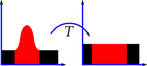
This method usually increases the global contrast of many images, especially when the usable data of the image is represented by close contrast values. Through this adjustment, the intensities can be better distributed on the histogram. This allows for areas of lower local contrast to gain a higher contrast. Histogram equalization accomplishes this by effectively spreading out the most frequent intensity values.

The method is useful in images with backgrounds and foregrounds that are both bright or both dark. In particular, the method can lead to better views of bone structure in x-ray images, and to better detail in photographs that are over or under-exposed. A key advantage of the method is that it is a fairly straightforward technique and an invertible operator. So in theory, if the histogram equalization function is known, then the original histogram can be recovered. The calculation is not computationally intensive. A disadvantage of the method is that it is indiscriminate. It may increase the contrast of background noise, while decreasing the usable signal.

In scientific imaging where spatial correlation is more important than intensity of signal (such as separating DNA fragments of quantized length), the small signal to noise ratio usually hampers visual detection.

Histogram equalization often produces unrealistic effects in photographs; however it is very useful for scientific images like thermal, satellite or x-ray images, often the same class of images to which one would apply false-color. Also histogram equalization can produce undesirable effects (like visible image gradient) when applied to images with low color depth. For example, if applied to 8-bit image displayed with 8-bit gray-scale palette it will further reduce color depth (number of unique shades of gray) of the image. Histogram equalization will work the best when applied to images with much higher color depth than palette size, like continuous data or 16-bit gray-scale images.

There are two ways to think about and implement histogram equalization, either as image change or as palette change. The operation can be expressed as P(M(I)) where I is the original image, M is histogram equalization mapping operation and P is a palette. If we define a new palette as P'=P(M) and leave image I unchanged then histogram equalization is implemented as palette change. On the other hand, if palette P remains unchanged and image is modified to I'=M(I) then the implementation is by image change. In most cases palette change is better as it preserves the original data.

Modifications of this method use multiple histograms, called subhistograms, to emphasize local contrast, rather than overall contrast. Examples of such methods include adaptive histogram equalization, contrast limiting adaptive histogram equalization or CLAHE, multipeak histogram equalization (MPHE), and multipurpose beta optimized bihistogram equalization (MBOBHE). The goal of these methods, especially MBOBHE, is to improve the contrast without producing brightness mean-shift and detail loss artifacts by modifying the HE algorithm.^[1]

A signal transform equivalent to histogram equalization also seems to happen in biological neural networks so as to maximize the output firing rate of the neuron as a function of the input statistics. This has been proved in particular in the fly retina.^[2]

Histogram equalization is a specific case of the more general class of histogram remapping methods. These methods seek to adjust the image to make it easier to analyze or improve visual quality (e.g., retinex)

Back projection

The back projection (or "project") of a histogrammed image is the re-application of the modified histogram to the original image, functioning as a look-up table for pixel brightness values.

For each group of pixels taken from the same position from all input single-channel images, the function puts the histogram bin value to the destination image, where the coordinates of the bin are determined by the values of pixels in this input group. In terms of statistics, the value of each output image pixel characterizes the probability that the corresponding input pixel group belongs to the object whose histogram is used.^[3]

Implementation

Consider a discrete grayscale image {x} and let n_i be the number of occurrences of gray level i. The probability of an occurrence of a pixel of level i in the image is

\ p_{x}(i)=p(x=i)={\frac {n_{i}}{n}},\quad 0\leq i<L

L being the total number of gray levels in the image (typically 256), n being the total number of pixels in the image, and $p_{x}(i)$ being in fact the image's histogram for pixel value i, normalized to [0,1].

Let us also define the cumulative distribution function corresponding to p_x as

\ cdf_{x}(i)=\sum _{j=0}^{i}p_{x}(j)

which is also the image's accumulated normalized histogram.

We would like to create a transformation of the form y = T(x) to produce a new image {y}, with a flat histogram. Such an image would have a linearized cumulative distribution function (CDF) across the value range, i.e.

\ cdf_{y}(i)=iK

for some constant K. The properties of the CDF allow us to perform such a transform (see Inverse distribution function); it is defined as

\ cdf_{y}(y^{\prime })=cdf_{y}(T(k))=cdf_{x}(k)

where k is in the range [0,L]). Notice that T maps the levels into the range [0,1], since we used a normalized histogram of {x}. In order to map the values back into their original range, the following simple transformation needs to be applied on the result:

\ y^{\prime }=y\cdot (\max\{x\}-\min\{x\})+\min\{x\}

A more detailed derivation is provided here.

Histogram equalization of color images

The above describes histogram equalization on a grayscale image. However it can also be used on color images by applying the same method separately to the Red, Green and Blue components of the RGB color values of the image. However, applying the same method on the Red, Green, and Blue components of an RGB image may yield dramatic changes in the image's color balance since the relative distributions of the color channels change as a result of applying the algorithm. However, if the image is first converted to another color space, Lab color space, or HSL/HSV color space in particular, then the algorithm can be applied to the luminance or value channel without resulting in changes to the hue and saturation of the image.^[4] There are several histogram equalization methods in 3D space. Trahanias and Venetsanopoulos applied histogram equalization in 3D color space^[5] However, it results in "whitening" where the probability of bright pixels are higher than that of dark ones.^[6] Han et al. proposed to use a new cdf defined by the iso-luminance plane, which results in uniform gray distribution.^[7]

Examples

For consistency with statistical usage, "CDF" (i.e. Cumulative distribution function) should be replaced by "cumulative histogram", especially since the article links to cumulative distribution function which is derived by dividing values in the cumulative histogram by the overall amount of pixels. The equalized CDF is defined in terms of rank as $rank/pixelcount$ .

Small image

The 8×8 sub-image shown in 8-bit grayscale

The 8-bit grayscale image shown has the following values:

{\begin{bmatrix}52&55&61&66&70&61&64&73\\63&59&55&90&109&85&69&72\\62&59&68&113&144&104&66&73\\63&58&71&122&154&106&70&69\\67&61&68&104&126&88&68&70\\79&65&60&70&77&68&58&75\\85&71&64&59&55&61&65&83\\87&79&69&68&65&76&78&94\end{bmatrix}}

The histogram for this image is shown in the following table. Pixel values that have a zero count are excluded for the sake of brevity.

Value	Count	Value	Count	Value	Count	Value	Count	Value	Count
52	1	64	2	72	1	85	2	113	1
55	3	65	3	73	2	87	1	122	1
58	2	66	2	75	1	88	1	126	1
59	3	67	1	76	1	90	1	144	1
60	1	68	5	77	1	94	1	154	1
61	4	69	3	78	1	104	2
62	1	70	4	79	2	106	1
63	2	71	2	83	1	109	1

The cumulative distribution function (cdf) is shown below. Again, pixel values that do not contribute to an increase in the cdf are excluded for brevity.

v, Pixel Intensity	cdf(v)	h(v), Equalized v
52	1	0
55	4	12
58	6	20
59	9	32
60	10	36
61	14	53
62	15	57
63	17	65
64	19	73
65	22	85
66	24	93
67	25	97
68	30	117
69	33	130
70	37	146
71	39	154
72	40	158
73	42	166
75	43	170
76	44	174
77	45	178
78	46	182
79	48	190
83	49	194
85	51	202
87	52	206
88	53	210
90	54	215
94	55	219
104	57	227
106	58	231
109	59	235
113	60	239
122	61	243
126	62	247
144	63	251
154	64	255

This cdf shows that the minimum value in the subimage is 52 and the maximum value is 154. The cdf of 64 for value 154 coincides with the number of pixels in the image. The cdf must be normalized to $[0,255]$ . The general histogram equalization formula is:

h(v)=\mathrm {round} \left({\frac {cdf(v)-cdf_{min}}{(M\times N)-1}}\times (L-1)\right)

where cdf_min is the minimum non-zero value of the cumulative distribution function (in this case 1), M × N gives the image's number of pixels (for the example above 64, where M is width and N the height) and L is the number of grey levels used (in most cases, like this one, 256).

Note that to scale values in the original data that are above 0 to the range 1 to L-1, inclusive, the above equation would instead be:

h(v)=\mathrm {round} \left({\frac {cdf(v)-cdf_{min}}{(M\times N)-1}}\times (L-2)\right)+1

where cdf(v) > 0. Scaling from 1 to 255 preserves the non-zero-ness of the minimum value.

The equalization formula for the example scaling data from 0 to 255, inclusive, is:

h(v)=\mathrm {round} \left({\frac {cdf(v)-1}{63}}\times 255\right)

For example, the cdf of 78 is 46. (The value of 78 is used in the bottom row of the 7th column.) The normalized value becomes

h(78)=\mathrm {round} \left({\frac {46-1}{63}}\times 255\right)=\mathrm {round} \left(0.714286\times 255\right)=182

Once this is done then the values of the equalized image are directly taken from the normalized cdf to yield the equalized values:

{\begin{bmatrix}0&12&53&93&146&53&73&166\\65&32&12&215&235&202&130&158\\57&32&117&239&251&227&93&166\\65&20&154&243&255&231&146&130\\97&53&117&227&247&210&117&146\\190&85&36&146&178&117&20&170\\202&154&73&32&12&53&85&194\\206&190&130&117&85&174&182&219\end{bmatrix}}

Notice that the minimum value (52) is now 0 and the maximum value (154) is now 255.


Original	Equalized


Histogram of Original image	Histogram of Equalized image

Full-sized image

An unequalized image	Corresponding histogram (red) and cumulative histogram (black)
The same image after histogram equalization	Corresponding histogram (red) and cumulative histogram (black)

Notes

↑ Hum, Yan Chai; Lai, Khin Wee; Mohamad Salim, Maheza Irna (11 October 2014). "Multiobjectives bihistogram equalization for image contrast enhancement". Complexity. 20 (2): 22–36. doi:10.1002/cplx.21499.
↑ Laughlin, S.B (1981). "A simple coding procedure enhances a neuron's information capacity". Z. Naturforsch. 9–10(36):910–2.
↑ Intel Corporation (2001). "Open Source Computer Vision Library Reference Manual" (PDF). Retrieved 2015-01-11.
↑ S. Naik and C. Murthy, "Hue-preserving color image enhancement without gamut problem," IEEE Trans. Image Processing, vol. 12, no. 12, pp. 1591–1598, Dec. 2003
↑ P. E. Trahanias and A. N. Venetsanopoulos, "Color image enhancement through 3-D histogram equalization," in Proc. 15th IAPR Int. Conf. Pattern Recognition, vol. 1, pp. 545–548, Aug.-Sep. 1992.
↑ N. Bassiou and C. Kotropoulos, "Color image histogram equalization by absolute discounting back-off," Computer Vision and Image Understanding, vol. 107, no. 1-2, pp.108-122, Jul.-Aug. 2007
↑ Ji-Hee Han, Sejung Yang, Byung-Uk Lee, "A Novel 3-D Color Histogram Equalization Method with Uniform 1-D Gray Scale Histogram", IEEE Trans. on Image Processing, Vol. 20, No. 2, pp. 506-512, Feb. 2011

References

Acharya and Ray, Image Processing: Principles and Applications, Wiley-Interscience 2005 ISBN 0-471-71998-6
Russ, The Image Processing Handbook: Fourth Edition, CRC 2002 ISBN 0-8493-2532-3

External links

This article is issued from Wikipedia - version of the 11/21/2016. The text is available under the Creative Commons Attribution/Share Alike but additional terms may apply for the media files.

Value	Count	Value	Count	Value	Count	Value	Count	Value	Count
52	1	64	2	72	1	85	2	113	1
55	3	65	3	73	2	87	1	122	1
58	2	66	2	75	1	88	1	126	1
59	3	67	1	76	1	90	1	144	1
60	1	68	5	77	1	94	1	154	1
61	4	69	3	78	1	104	2
62	1	70	4	79	2	106	1
63	2	71	2	83	1	109	1

v, Pixel Intensity	cdf(v)	h(v), Equalized v
52	1	0
55	4	12
58	6	20
59	9	32
60	10	36
61	14	53
62	15	57
63	17	65
64	19	73
65	22	85
66	24	93
67	25	97
68	30	117
69	33	130
70	37	146
71	39	154
72	40	158
73	42	166
75	43	170
76	44	174
77	45	178
78	46	182
79	48	190
83	49	194
85	51	202
87	52	206
88	53	210
90	54	215
94	55	219
104	57	227
106	58	231
109	59	235
113	60	239
122	61	243
126	62	247
144	63	251
154	64	255

Value	Count	Value	Count	Value	Count	Value	Count	Value	Count
52	1	64	2	72	1	85	2	113	1
55	3	65	3	73	2	87	1	122	1
58	2	66	2	75	1	88	1	126	1
59	3	67	1	76	1	90	1	144	1
60	1	68	5	77	1	94	1	154	1
61	4	69	3	78	1	104	2
62	1	70	4	79	2	106	1
63	2	71	2	83	1	109	1

v, Pixel Intensity	cdf(v)	h(v), Equalized v
52	1	0
55	4	12
58	6	20
59	9	32
60	10	36
61	14	53
62	15	57
63	17	65
64	19	73
65	22	85
66	24	93
67	25	97
68	30	117
69	33	130
70	37	146
71	39	154
72	40	158
73	42	166
75	43	170
76	44	174
77	45	178
78	46	182
79	48	190
83	49	194
85	51	202
87	52	206
88	53	210
90	54	215
94	55	219
104	57	227
106	58	231
109	59	235
113	60	239
122	61	243
126	62	247
144	63	251
154	64	255