Grad–Shafranov equation
The Grad–Shafranov equation (H. Grad and H. Rubin (1958); Vitalii Dmitrievich Shafranov (1966)) is the equilibrium equation in ideal magnetohydrodynamics (MHD) for a two dimensional plasma, for example the axisymmetric toroidal plasma in a tokamak. This equation is a two-dimensional, nonlinear, elliptic partial differential equation obtained from the reduction of the ideal MHD equations to two dimensions, often for the case of toroidal axisymmetry (the case relevant in a tokamak). The flux function  is both a dependent and an independent variable in this equation:
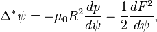
where  is the magnetic permeability,
  is the pressure,
 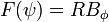 and the magnetic field and current are, respectively, given by

The elliptic operator  is
is
 .
.
The nature of the equilibrium, whether it be a tokamak, reversed field pinch, etc. is largely determined by the choices of the two functions  and as well as the boundary conditions.
Derivation (in slab coordinates)
In the following, it is assumed that the system is 2-dimensional with  as the invariant axis, i.e.
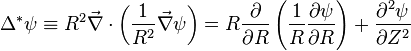
  for all quantities. Then the magnetic field can be written in cartesian coordinates as
or more compactly,
where  is the vector potential for the in-plane (x and y components) magnetic field. Note that based on this form for B we can see that A is constant along any given magnetic field line, since
  is everywhere perpendicular to B. (Also note that -A is the flux function mentioned above.)
Two dimensional, stationary, magnetic structures are described by the balance of pressure forces and magnetic forces, i.e.:
where p is the plasma pressure and j is the electric current. It is known that p is a constant along any field line, (again since  is everywhere perpendicular to B). Additionally, the two-dimensional assumption () means that the z- component of the left hand side must be zero, so the z-component of the magnetic force on the right hand side must also be zero. This means that
  , i.e.
  is parallel to
  .
.
The right hand side of the previous equation can be considered in two parts:

where the  subscript denotes the component in the plane perpendicular to the -axis. The component of the current in the above equation can be written in terms of the one-dimensional vector potential as
 .
.
The in plane field is
 ,
,
and using Maxwell–Ampère's equation, the in plane current is given by
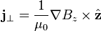 .
.
In order for this vector to be parallel to as required, the vector  must be perpendicular to , and
  must therefore, like
  , be a field-line invariant.
Rearranging the cross products above leads to
 ,
,
and

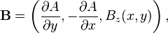
These results can be substituted into the expression for to yield:
![\nabla p = -\left[\frac{1}{\mu_0} \nabla^2 A\right]\nabla A - \frac{1}{\mu_0} B_z\nabla B_z.](../I/m/176c44868231d6b8aefd261c711814ac.png)
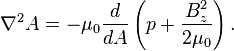
Since and are constants along a field line, and functions only of  , hence
 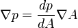 and
and 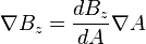 . Thus, factoring out and rearranging terms yields the Grad–Shafranov equation:
References
- Grad, H., and Rubin, H. (1958) Hydromagnetic Equilibria and Force-Free Fields. Proceedings of the 2nd UN Conf. on the Peaceful Uses of Atomic Energy, Vol. 31, Geneva: IAEA p. 190.
- Shafranov, V.D. (1966) Plasma equilibrium in a magnetic field, Reviews of Plasma Physics, Vol. 2, New York: Consultants Bureau, p. 103.
- Woods, Leslie C. (2004) Physics of plasmas, Weinheim: WILEY-VCH Verlag GmbH & Co. KGaA, chapter 2.5.4
- Haverkort, J.W. (2009) Axisymmetric Ideal MHD Tokamak Equilibria. Notes about the Grad-Shafranov equation, selected aspects of the equation and its analytical solutions.
- Haverkort, J.W. (2009) Axisymmetric Ideal MHD equilibria with Toroidal Flow. Incorporation of toroidal flow, relation to kinetic and two-fluid models, and discussion of specific analytical solutions.