Godunov's theorem
In numerical analysis and computational fluid dynamics, Godunov's theorem — also known as Godunov's order barrier theorem — is a mathematical theorem important in the development of the theory of high resolution schemes for the numerical solution of partial differential equations.
The theorem states that:
- Linear numerical schemes for solving partial differential equations (PDE's), having the property of not generating new extrema (monotone scheme), can be at most first-order accurate.
Professor Sergei K. Godunov originally proved the theorem as a Ph.D. student at Moscow State University. It is his most influential work in the area of applied and numerical mathematics and has had a major impact on science and engineering, particularly in the development of methods used in computational fluid dynamics (CFD) and other computational fields. One of his major contributions was to prove the theorem (Godunov, 1954; Godunov, 1959), that bears his name.
The theorem
We generally follow Wesseling (2001).
Aside
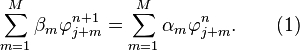
Assume a continuum problem described by a PDE is to be computed using a numerical scheme based upon a uniform computational grid and a one-step, constant step-size, M grid point, integration algorithm, either implicit or explicit. Then if  and
and  , such a scheme can be described by
In other words, the solution  at time
  and location
  is a linear function of the solution at the previous time step
  . We assume that
  determines uniquely. Now, since the above equation represents a linear relationship between
  and we can perform a linear transformation to obtain the following equivalent form,
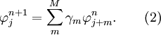
Theorem 1: Monotonicity preserving
The above scheme of equation (2) is monotonicity preserving if and only if
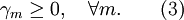
Proof - Godunov (1959)
Case 1: (sufficient condition)
Assume (3) applies and that  is monotonically increasing with
  .
.
Then, because 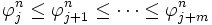 it therefore follows that
 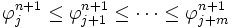 because
This means that monotonicity is preserved for this case.
Case 2: (necessary condition)
We prove the necessary condition by contradiction. Assume that  for some
  and choose the following monotonically increasing
  ,
,

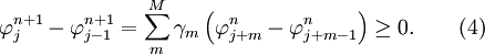
Then from equation (2) we get
![\varphi _j^{n + 1} - \varphi _{j-1}^{n+1} = \sum\limits_m^M {\gamma _m } \left( {\varphi _{j + m}^{n} - \varphi _{j + m - 1}^{n} } \right) = \left\{ {\begin{array}{*{20}c}
{0,} & {\left[ {j + m \ne k} \right]} \\
{\gamma _m ,} & {\left[ {j + m = k} \right]} \\
\end{array}} \right . \quad \quad ( 6)](../I/m/ce0ac9e056c71c1d352f261c85678589.png)
Now choose  , to give

which implies that is NOT increasing, and we have a contradiction. Thus, monotonicity is NOT preserved for  , which completes the proof.
Theorem 2: Godunov’s Order Barrier Theorem
Linear one-step second-order accurate numerical schemes for the convection equation
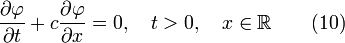
cannot be monotonicity preserving unless
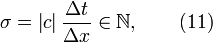
where  is the signed Courant–Friedrichs–Lewy condition (CFL) number.
Proof - Godunov (1959)
Assume a numerical scheme of the form described by equation (2) and choose

The exact solution is
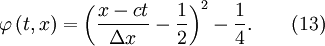
If we assume the scheme to be at least second-order accurate, it should produce the following solution exactly

Substituting into equation (2) gives:
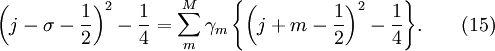
Suppose that the scheme IS monotonicity preserving, then according to the theorem 1 above,  .
.
Now, it is clear from equation (15) that
Assume 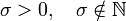 and choose such that
  . This implies that
  and
and  .
.
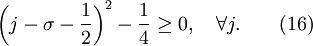
It therefore follows that,
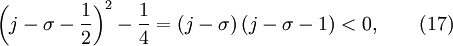
which contradicts equation (16) and completes the proof.
The exceptional situation whereby  is only of theoretical interest, since this cannot be realised with variable coefficients. Also, integer CFL numbers greater than unity would not be feasible for practical problems.
See also
References
- Godunov, Sergei K. (1954), Ph.D. Dissertation: Different Methods for Shock Waves, Moscow State University.
- Godunov, Sergei K. (1959), A Difference Scheme for Numerical Solution of Discontinuous Solution of Hydrodynamic Equations, Math. Sbornik, 47, 271-306, translated US Joint Publ. Res. Service, JPRS 7226, 1969.
- Wesseling, Pieter (2001), Principles of Computational Fluid Dynamics, Springer-Verlag.
Further reading
- Hirsch, C. (1990), Numerical Computation of Internal and External Flows, vol 2, Wiley.
- Laney, Culbert B. (1998), Computational Gas Dynamics, Cambridge University Press.
- Toro, E. F. (1999), Riemann Solvers and Numerical Methods for Fluid Dynamics, Springer-Verlag.
- Tannehill, John C., et al., (1997), Computational Fluid mechanics and Heat Transfer, 2nd Ed., Taylor and Francis.