Gent (hyperelastic model)
| Continuum mechanics | ||||
|---|---|---|---|---|
 | ||||
|
Laws
|
||||
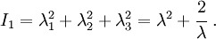
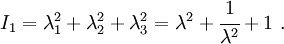
The Gent hyperelastic material model [1] is a phenomenological model of rubber elasticity that is based on the concept of limiting chain extensibility. In this model, the strain energy density function is designed such that it has a singularity when the first invariant of the left Cauchy-Green deformation tensor reaches a limiting value  .
.
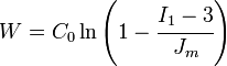
The strain energy density function for the Gent model is [1]
where  is the shear modulus and
  .
.
In the limit where  , the Gent model reduces to the Neo-Hookean solid model. This can be seen by expressing the Gent model in the form
![W = \cfrac{\mu}{2x}\ln\left[1 - (I_1-3)x\right] ~;~~ x := \cfrac{1}{J_m}](../I/m/2a39397e1f6ee9b463a73cdb64f0576f.png)
A Taylor series expansion of ![\ln\left[1 - (I_1-3)x\right]](../I/m/ae694f827150ed6bd90df278d7489bea.png) around
around  and taking the limit as
  leads to
which is the expression for the strain energy density of a Neo-Hookean solid.
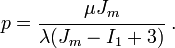
Several compressible versions of the Gent model have been designed. One such model has the form[2]
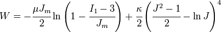
where  ,
,  is the bulk modulus, and
  is the deformation gradient.
Consistency condition
We may alternatively express the Gent model in the form
For the model to be consistent with linear elasticity, the following condition has to be satisfied:
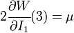
where is the shear modulus of the material.
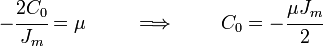
Now, at  ,
,
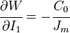
Therefore, the consistency condition for the Gent model is
The Gent model assumes that 
Stress-deformation relations
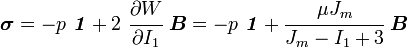
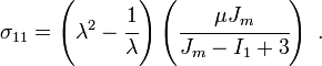
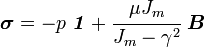
The Cauchy stress for the incompressible Gent model is given by
Uniaxial extension

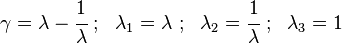
For uniaxial extension in the  -direction, the principal stretches are
 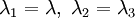 . From incompressibility
 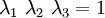 . Hence
  .
Therefore,
.
Therefore,
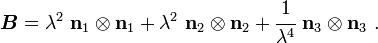
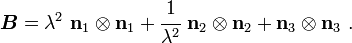
The left Cauchy-Green deformation tensor can then be expressed as
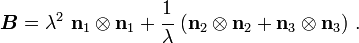
If the directions of the principal stretches are oriented with the coordinate basis vectors, we have

If  , we have
Therefore,
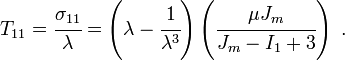
The engineering strain is  . The engineering stress is
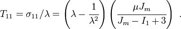
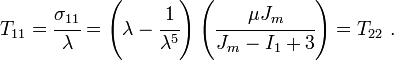
Equibiaxial extension
For equibiaxial extension in the and  directions, the principal stretches are
 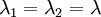 . From incompressibility . Hence
  .
Therefore,
.
Therefore,
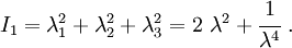
The left Cauchy-Green deformation tensor can then be expressed as
If the directions of the principal stretches are oriented with the coordinate basis vectors, we have
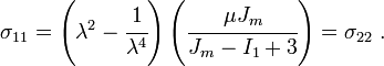
The engineering strain is . The engineering stress is
Planar extension
Planar extension tests are carried out on thin specimens which are constrained from deforming in one direction. For planar extension in the directions with the  direction constrained, the principal stretches are
 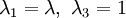 . From incompressibility . Hence
  .
Therefore,
.
Therefore,
The left Cauchy-Green deformation tensor can then be expressed as
If the directions of the principal stretches are oriented with the coordinate basis vectors, we have

The engineering strain is . The engineering stress is
Simple shear
The deformation gradient for a simple shear deformation has the form[3]

where  are reference orthonormal basis vectors in the plane of deformation and the shear deformation is given by
In matrix form, the deformation gradient and the left Cauchy-Green deformation tensor may then be expressed as
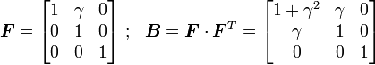
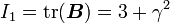
Therefore,
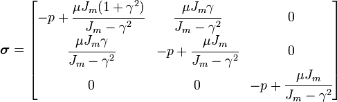
and the Cauchy stress is given by
In matrix form,
References
- ↑ 1.0 1.1 Gent, A.N., 1996, A new constitutive relation for rubber, Rubber Chemistry Tech., 69, pp. 59-61.
- ↑ Mac Donald, B. J., 2007, Practical stress analysis with finite elements, Glasnevin, Ireland.
- ↑ Ogden, R. W., 1984, Non-linear elastic deformations, Dover.
See also
- Hyperelastic material
- Strain energy density function
- Mooney-Rivlin solid
- Finite strain theory
- Stress measures