Generalized normal distribution

The generalized normal distribution or generalized Gaussian distribution (GGD) is either of two families of parametric continuous probability distributions on the real line. Both families add a shape parameter to the normal distribution. To distinguish the two families, they are referred to below as "version 1" and "version 2". However this is not a standard nomenclature.

Version 1

Generalized Normal (version 1)
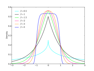
Probability density function
Cumulative distribution function
Parameters	$\mu \,$ location (real) $\alpha \,$ scale (positive, real) $\beta \,$ shape (positive, real)
Support	$x\in (-\infty ;+\infty )\!$
PDF	$\frac{\beta}{2\alpha\Gamma(1/\beta)} \; e^{-(\|x-\mu\|/\alpha)^\beta}$ $\Gamma$ denotes the gamma function
CDF	$\frac{1}{2} + \sgn(x-\mu)\frac{\gamma\left[1/\beta, \left( \frac{\|x-\mu\|}{\alpha} \right)^\beta\right]}{2\Gamma(1/\beta)}$ $\gamma$ denotes the lower incomplete gamma function
Mean	$\mu \,$
Median	$\mu \,$
Mode	$\mu \,$
Variance	$\frac{\alpha^2\Gamma(3/\beta)}{\Gamma(1/\beta)}$
Skewness	0
Ex. kurtosis	$\frac{\Gamma(5/\beta)\Gamma(1/\beta)}{\Gamma(3/\beta)^2}-3$
Entropy	$\frac{1}{\beta}-\log\left[\frac{\beta}{2\alpha\Gamma(1/\beta)}\right]$ ^[1]

Known also as the exponential power distribution, or the generalized error distribution, this is a parametric family of symmetric distributions. It includes all normal and Laplace distributions, and as limiting cases it includes all continuous uniform distributions on bounded intervals of the real line.

This family includes the normal distribution when $\textstyle\beta=2$ (with mean $\textstyle\mu$ and variance $\textstyle \frac{\alpha^2}{2}$ ) and it includes the Laplace distribution when $\textstyle\beta=1$ . As $\textstyle\beta\rightarrow\infty$ , the density converges pointwise to a uniform density on $\textstyle (\mu-\alpha,\mu+\alpha)$ .

This family allows for tails that are either heavier than normal (when $\beta<2$ ) or lighter than normal (when $\beta>2$ ). It is a useful way to parametrize a continuum of symmetric, platykurtic densities spanning from the normal ( $\textstyle\beta=2$ ) to the uniform density ( $\textstyle\beta=\infty$ ), and a continuum of symmetric, leptokurtic densities spanning from the Laplace ( $\textstyle\beta=1$ ) to the normal density ( $\textstyle\beta=2$ ).

Parameter estimation

Parameter estimation via maximum likelihood and the method of moments has been studied.^[2] The estimates do not have a closed form and must be obtained numerically. Estimators that do not require numerical calculation have also been proposed.^[3]

The generalized normal log-likelihood function has infinitely many continuous derivates (i.e. it belongs to the class C^∞ of smooth functions) only if $\textstyle\beta$ is a positive, even integer. Otherwise, the function has $\textstyle\lfloor \beta \rfloor$ continuous derivatives. As a result, the standard results for consistency and asymptotic normality of maximum likelihood estimates of $\beta$ only apply when $\textstyle\beta\ge 2$ .

Maximum likelihood estimator

It is possible to fit the generalized normal distribution adopting an approximate maximum likelihood method.^[4]^[5] With $\mu$ initially set to the sample first moment $m_{1}$ , $\textstyle\beta$ is estimated by using a Newton–Raphson iterative procedure, starting from an initial guess of $\textstyle\beta=\textstyle\beta_0$ ,

\beta _0 = \frac{m_1}{\sqrt{m_2}},

where

m_1={1 \over N} \sum_{i=1}^N |x_i|,

is the first statistical moment of the absolute values and $m_{2}$ is the second statistical moment. The iteration is

\beta _{i+1} = \beta _{i} - \frac{g(\beta _{i})}{g'(\beta _{i})} ,

where

g(\beta )=1+{\frac {\psi (1/\beta )}{\beta }}-{\frac {\sum _{i=1}^{N}|x_{i}-\mu |^{\beta }\log |x_{i}-\mu |}{\sum _{i=1}^{N}|x_{i}-\mu |^{\beta }}}+{\frac {\log({\frac {\beta }{N}}\sum _{i=1}^{N}|x_{i}-\mu |^{\beta })}{\beta }},

and

{\begin{aligned}g'(\beta )={}&-{\frac {\psi (1/\beta )}{\beta ^{2}}}-{\frac {\psi '(1/\beta )}{\beta ^{3}}}+{\frac {1}{\beta ^{2}}}-{\frac {\sum _{i=1}^{N}|x_{i}-\mu |^{\beta }(\log |x_{i}-\mu |)^{2}}{\sum _{i=1}^{N}|x_{i}-\mu |^{\beta }}}\\[6pt]&{}+{\frac {\left(\sum _{i=1}^{N}|x_{i}-\mu |^{\beta }\log |x_{i}-\mu |\right)^{2}}{\left(\sum _{i=1}^{N}|x_{i}-\mu |^{\beta }\right)^{2}}}+{\frac {\sum _{i=1}^{N}|x_{i}-\mu |^{\beta }\log |x_{i}-\mu |}{\beta \sum _{i=1}^{N}|x_{i}-\mu |^{\beta }}}\\[6pt]&{}-{\frac {\log \left({\frac {\beta }{N}}\sum _{i=1}^{N}|x_{i}-\mu |^{\beta }\right)}{\beta ^{2}}},\end{aligned}}

and where $\psi$ and $\psi '$ are the digamma function and trigamma function.

Given a value for $\textstyle\beta$ , it is possible to estimate $\mu$ by finding the minimum of:

\min _{\mu }=\sum _{i=1}^{N}|x_{i}-\mu |^{\beta }

Finally $\textstyle\alpha$ is evaluated as

\alpha =\left({\frac {\beta }{N}}\sum _{i=1}^{N}|x_{i}-\mu |^{\beta }\right)^{1/\beta }.

Applications

This version of the generalized normal distribution has been used in modeling when the concentration of values around the mean and the tail behavior are of particular interest.^[6]^[7] Other families of distributions can be used if the focus is on other deviations from normality. If the symmetry of the distribution is the main interest, the skew normal family or version 2 of the generalized normal family discussed below can be used. If the tail behavior is the main interest, the student t family can be used, which approximates the normal distribution as the degrees of freedom grows to infinity. The t distribution, unlike this generalized normal distribution, obtains heavier than normal tails without acquiring a cusp at the origin.

Properties

The multivariate generalized normal distribution, i.e. the product of $n$ exponential power distributions with the same $\beta$ and $\alpha$ parameters, is the only probability density that can be written in the form $p(\mathbf x)=g(\|\mathbf x\|_\beta)$ and has independent marginals.^[8] The results for the special case of the Multivariate normal distribution is originally attributed to Maxwell.^[9]

Version 2

Generalized Normal (version 2)
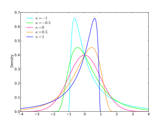
Probability density function
Cumulative distribution function
Parameters	$\xi \,$ location (real) $\alpha \,$ scale (positive, real) $\kappa \,$ shape (real)
Support	$x \in (-\infty,\xi+\alpha/\kappa) \text{ if } \kappa>0$ $x \in (-\infty,\infty) \text{ if } \kappa=0$ $x \in (\xi+\alpha/\kappa; +\infty) \text{ if } \kappa<0$
PDF	$\frac{\phi(y)}{\alpha-\kappa(x-\xi)}$ , where $y = \begin{cases} - \frac{1}{\kappa} \log \left[ 1- \frac{\kappa(x-\xi)}{\alpha} \right] & \text{if } \kappa \neq 0 \\ \frac{x-\xi}{\alpha} & \text{if } \kappa=0 \end{cases}$ $\phi$ is the standard normal pdf
CDF	$\Phi(y)$ , where $y = \begin{cases} - \frac{1}{\kappa} \log \left[ 1- \frac{\kappa(x-\xi)}{\alpha} \right] & \text{if } \kappa \neq 0 \\ \frac{x-\xi}{\alpha} & \text{if } \kappa=0 \end{cases}$ $\Phi$ is the standard normal CDF
Mean	$\xi - \frac{\alpha}{\kappa} \left( e^{\kappa^2/2} - 1 \right)$
Median	$\xi \,$
Variance	$\frac{\alpha^2}{\kappa^2} e^{\kappa^2} \left( e^{\kappa^2} - 1 \right)$
Skewness	$\frac{3 e^{\kappa^2} - e^{3 \kappa^2} - 2}{(e^{\kappa^2} - 1)^{3/2}} \text{ sign}(\kappa)$
Ex. kurtosis	$e^{4 \kappa^2} + 2 e^{3 \kappa^2} + 3 e^{2 \kappa^2} - 6$

This is a family of continuous probability distributions in which the shape parameter can be used to introduce skew.^[10]^[11] When the shape parameter is zero, the normal distribution results. Positive values of the shape parameter yield left-skewed distributions bounded to the right, and negative values of the shape parameter yield right-skewed distributions bounded to the left. Only when the shape parameter is zero is the density function for this distribution positive over the whole real line: in this case the distribution is a normal distribution, otherwise the distributions are shifted and possibly reversed log-normal distributions.

Parameter estimation

Parameters can be estimated via maximum likelihood estimation or the method of moments. The parameter estimates do not have a closed form, so numerical calculations must be used to compute the estimates. Since the sample space (the set of real numbers where the density is non-zero) depends on the true value of the parameter, some standard results about the performance of parameter estimates will not automatically apply when working with this family.

Applications

This family of distributions can be used to model values that may be normally distributed, or that may be either right-skewed or left-skewed relative to the normal distribution. The skew normal distribution is another distribution that is useful for modeling deviations from normality due to skew. Other distributions used to model skewed data include the gamma, lognormal, and Weibull distributions, but these do not include the normal distributions as special cases.

Other distributions related to the normal

The two generalized normal families described here, like the skew normal family, are parametric families that extends the normal distribution by adding a shape parameter. Due to the central role of the normal distribution in probability and statistics, many distributions can be characterized in terms of their relationship to the normal distribution. For example, the lognormal, folded normal, and inverse normal distributions are defined as transformations of a normally-distributed value, but unlike the generalized normal and skew-normal families, these do not include the normal distributions as special cases.
Actually all distributions with finite variance are in the limit highly related to the normal distribution. The Student-t distribution, the Irwin–Hall distribution and the Bates distribution also extend the normal distribution, and include in the limit the normal distribution. So there is no strong reason to prefer the "generalized" normal distribution of type 1, e.g. over a combination of Student-t and a normalized extended Irwin–Hall – this would include e.g. the triangular distribution (which cannot be modeled by the generalized Gaussian type 1).
A symmetric distribution which can model both tail (long and short) and center behavior (like flat, triangular or Gaussian) completely independently could be derived e.g. by using X = IH/chi.

References

↑ Nadarajah, Saralees (September 2005). "A generalized normal distribution". Journal of Applied Statistics. 32 (7): 685–694. doi:10.1080/02664760500079464.
↑ Varanasi, M.K.; Aazhang, B. (October 1989). "Parametric generalized Gaussian density estimation". Journal of the Acoustical Society of America. 86 (4): 1404–1415. doi:10.1121/1.398700.
↑ Domínguez-Molina, J. Armando; González-Farías, Graciela; Rodríguez-Dagnino, Ramón M. "A practical procedure to estimate the shape parameter in the generalized Gaussian distribution" (PDF). Retrieved 2009-03-03.
↑ Varanasi, M.K.; Aazhang B. (1989). "Parametric generalized Gaussian density estimation". J. Acoust. Soc. Am. 86: 1404–1415. doi:10.1121/1.398700.
↑ Do, M.N.; Vetterli, M. (February 2002). "Wavelet-based Texture Retrieval Using Generalised Gaussian Density and Kullback-Leibler Distance". Transaction on Image Processing. 11: 146–158. doi:10.1109/83.982822.
↑ Liang, Faming; Liu, Chuanhai; Wang, Naisyin (April 2007). "A robust sequential Bayesian method for identification of differentially expressed genes". Statistica Sinica. 17 (2): 571–597. Retrieved 2009-03-03.
↑ Box, George E. P.; Tiao, George C. (1992). Bayesian Inference in Statistical Analysis. New York: Wiley. ISBN 0-471-57428-7.
↑ Sinz, Fabian; Gerwinn, Sebastian; Bethge, Matthias (May 2009). "Characterization of the p-Generalized Normal Distribution.". Journal of Multivariate Analysis. 100 (5): 817–820. doi:10.1016/j.jmva.2008.07.006.
↑ Kac, M. (1939). "On a characterization of the normal distribution". American Journal of Mathematics. 61 (3): 726–728. doi:10.2307/2371328.
↑ Hosking, J.R.M., Wallis, J.R. (1997) Regional frequency analysis: an approach based on L-moments, Cambridge University Press. ISBN 0-521-43045-3. Section A.8
↑ Documentation for the lmomco R package

Probability distributions

List

Discrete univariate with finite support	Benford Bernoulli beta-binomial binomial categorical hypergeometric Poisson binomial Rademacher discrete uniform Zipf Zipf–Mandelbrot

Discrete univariate with infinite support	beta negative binomial Borel Conway–Maxwell–Poisson discrete phase-type Delaporte extended negative binomial Gauss–Kuzmin geometric logarithmic negative binomial parabolic fractal Poisson Skellam Yule–Simon zeta

Continuous univariate supported on a bounded interval	arcsine ARGUS Balding–Nichols Bates beta beta rectangular Irwin–Hall Kumaraswamy logit-normal noncentral beta raised cosine reciprocal triangular U-quadratic uniform Wigner semicircle

Continuous univariate supported on a semi-infinite interval	Benini Benktander 1st kind Benktander 2nd kind beta prime Burr chi-squared chi Dagum Davis exponential-logarithmic Erlang exponential F folded normal Flory–Schulz Fréchet gamma gamma/Gompertz generalized inverse Gaussian Gompertz half-logistic half-normal Hotelling's T-squared hyper-Erlang hyperexponential hypoexponential inverse chi-squared scaled inverse chi-squared inverse Gaussian inverse gamma Kolmogorov Lévy log-Cauchy log-Laplace log-logistic log-normal Lomax matrix-exponential Maxwell–Boltzmann Maxwell–Jüttner Mittag-Leffler Nakagami noncentral chi-squared Pareto phase-type poly-Weibull Rayleigh relativistic Breit–Wigner Rice shifted Gompertz truncated normal type-2 Gumbel Weibull Discrete Weibull Wilks's lambda

Continuous univariate supported on the whole real line	Cauchy exponential power Fisher's z Gaussian q generalized normal generalized hyperbolic geometric stable Gumbel Holtsmark hyperbolic secant Johnson's S_U Landau Laplace asymmetric Laplace logistic noncentral t normal (Gaussian) normal-inverse Gaussian skew normal slash stable Student's t type-1 Gumbel Tracy–Widom variance-gamma Voigt

Continuous univariate with support whose type varies	generalized extreme value generalized Pareto Tukey lambda q-Gaussian q-exponential q-Weibull shifted log-logistic

Mixed continuous-discrete univariate	rectified Gaussian

Multivariate (joint)	Discrete Ewens multinomial Dirichlet-multinomial negative multinomial Continuous Dirichlet generalized Dirichlet multivariate normal multivariate stable multivariate t normal-inverse-gamma normal-gamma Matrix-valued inverse matrix gamma inverse-Wishart matrix normal matrix t matrix gamma normal-inverse-Wishart normal-Wishart Wishart

Directional	Univariate (circular) directional Circular uniform univariate von Mises wrapped normal wrapped Cauchy wrapped exponential wrapped asymmetric Laplace wrapped Lévy Bivariate (spherical) Kent Bivariate (toroidal) bivariate von Mises Multivariate von Mises–Fisher Bingham

Degenerate and singular	Degenerate Dirac delta function Singular Cantor

Families	Circular compound Poisson elliptical exponential natural exponential location-scale maximum entropy mixture Pearson Tweedie wrapped

Statistics

Descriptive statistics

Continuous data

Center	Mean arithmetic geometric harmonic Median Mode

Dispersion	Variance Standard deviation Coefficient of variation Percentile Range Interquartile range

Shape	Moments Skewness Kurtosis L-moments

Count data

Index of dispersion

Summary tables

Dependence

Graphics

Data collection

Study design	Population Statistic Effect size Statistical power Sample size determination Missing data

Survey methodology	Sampling Standard error stratified cluster Opinion poll Questionnaire

Controlled experiments	Design control optimal Controlled trial Randomized Random assignment Replication Blocking Interaction Factorial experiment

Uncontrolled studies	Observational study Natural experiment Quasi-experiment

Statistical inference

Statistical theory

Frequentist inference

Point estimation	Estimating equations Maximum likelihood Method of moments M-estimator Minimum distance Unbiased estimators Mean-unbiased minimum-variance Rao–Blackwellization Lehmann–Scheffé theorem Median unbiased Plug-in

Interval estimation	Confidence interval Pivot Likelihood interval Prediction interval Tolerance interval Resampling Bootstrap Jackknife

Testing hypotheses	1- & 2-tails Power Uniformly most powerful test Permutation test Randomization test Multiple comparisons

Parametric tests	Likelihood-ratio Wald Score

Specific tests

Z (normal) Student's t-test F

Goodness of fit	Chi-squared Kolmogorov–Smirnov Anderson–Darling Normality (Shapiro–Wilk) Likelihood-ratio test Model selection Cross validation AIC BIC

Rank statistics	Sign Sample median Signed rank (Wilcoxon) Hodges–Lehmann estimator Rank sum (Mann–Whitney) Nonparametric anova 1-way (Kruskal–Wallis) 2-way (Friedman) Ordered alternative (Jonckheere–Terpstra)

Bayesian inference

Correlation	Pearson product–moment Partial correlation Confounding variable Coefficient of determination

Regression analysis	Errors and residuals Regression model validation Mixed effects models Simultaneous equations models Multivariate adaptive regression splines (MARS)

Linear regression	Simple linear regression Ordinary least squares General linear model Bayesian regression

Non-standard predictors	Nonlinear regression Nonparametric Semiparametric Isotonic Robust Heteroscedasticity Homoscedasticity

Generalized linear model	Exponential families Logistic (Bernoulli) / Binomial / Poisson regressions

Partition of variance	Analysis of variance (ANOVA, anova) Analysis of covariance Multivariate ANOVA Degrees of freedom

Categorical / Multivariate / Time-series / Survival analysis

Categorical

Multivariate

Time-series

General	Decomposition Trend Stationarity Seasonal adjustment Exponential smoothing Cointegration Structural break Granger causality

Specific tests	Dickey–Fuller Johansen Q-statistic (Ljung–Box) Durbin–Watson Breusch–Godfrey

Time domain	Autocorrelation (ACF) partial (PACF) Cross-correlation (XCF) ARMA model ARIMA model (Box–Jenkins) Autoregressive conditional heteroskedasticity (ARCH) Vector autoregression (VAR)

Frequency domain	Spectral density estimation Fourier analysis Wavelet

Survival

Survival function	Kaplan–Meier estimator (product limit) Proportional hazards models Accelerated failure time (AFT) model First hitting time

Hazard function	Nelson–Aalen estimator

Test	Log-rank test

Applications

Biostatistics	Bioinformatics Clinical trials / studies Epidemiology Medical statistics

Engineering statistics	Chemometrics Methods engineering Probabilistic design Process / quality control Reliability System identification

Social statistics	Actuarial science Census Crime statistics Demography Econometrics National accounts Official statistics Population statistics Psychometrics

Spatial statistics	Cartography Environmental statistics Geographic information system Geostatistics Kriging

Category
Portal
Commons
WikiProject

This article is issued from Wikipedia - version of the 11/23/2016. The text is available under the Creative Commons Attribution/Share Alike but additional terms may apply for the media files.

Generalized normal distribution

Version 1

Parameter estimation

Maximum likelihood estimator

Applications

Properties

Version 2

Parameter estimation

Applications

Other distributions related to the normal

See also

References