Divergence theorem
| Part of a series of articles about | ||||||
| Calculus | ||||||
|---|---|---|---|---|---|---|
|
||||||
|
Specialized |
||||||
In vector calculus, the divergence theorem, also known as Gauss's theorem or Ostrogradsky's theorem,[1][2] is a result that relates the flow (that is, flux) of a vector field through a surface to the behavior of the vector field inside the surface.
More precisely, the divergence theorem states that the outward flux of a vector field through a closed surface is equal to the volume integral of the divergence over the region inside the surface. Intuitively, it states that the sum of all sources minus the sum of all sinks gives the net flow out of a region.
The divergence theorem is an important result for the mathematics of engineering, in particular in electrostatics and fluid dynamics.
In physics and engineering, the divergence theorem is usually applied in three dimensions. However, it generalizes to any number of dimensions. In one dimension, it is equivalent to the fundamental theorem of calculus. In two dimensions, it is equivalent to Green's theorem.
The theorem is a special case of the more general Stokes' theorem.[3]
Intuition
If a fluid is flowing in some area, then the rate at which fluid flows out of a certain region within that area can be calculated by adding up the sources inside the region and subtracting the sinks. The fluid flow is represented by a vector field, and the vector field's divergence at a given point describes the strength of the source or sink there. So, integrating the field's divergence over the interior of the region should equal the integral of the vector field over the region's boundary. The divergence theorem says that this is true.[4]
The divergence theorem is employed in any conservation law which states that the volume total of all sinks and sources, that is the volume integral of the divergence, is equal to the net flow across the volume's boundary.[5]
Mathematical statement
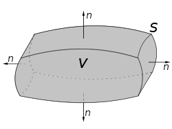
Suppose V is a subset of (in the case of n = 3, V represents a volume in 3D space) which is compact and has a piecewise smooth boundary S (also indicated with ∂V = S ). If F is a continuously differentiable vector field defined on a neighborhood of V, then we have:[6]


The left side is a volume integral over the volume V, the right side is the surface integral over the boundary of the volume V. The closed manifold ∂V is quite generally the boundary of V oriented by outward-pointing normals, and n is the outward pointing unit normal field of the boundary ∂V. (dS may be used as a shorthand for ndS.) The symbol within the two integrals stresses once more that ∂V is a closed surface. In terms of the intuitive description above, the left-hand side of the equation represents the total of the sources in the volume V, and the right-hand side represents the total flow across the boundary S.
Corollaries
By replacing in the divergence theorem with specific forms, other useful identities can be derived (cf. vector identities).[6]

- With for a scalar function g and a vector field F,

![\iiint _{V}\left[\mathbf {F} \cdot \left(\nabla g\right)+g\left(\nabla \cdot \mathbf {F} \right)\right]dV=](../I/m/bce62e824c35adc06d6e27eb7c6cb6104bc69ed2.svg)

- A special case of this is F = ∇ f , in which case the theorem is the basis for Green's identities.
- With for two vector fields F and G,

![\iiint _{V}\left[\mathbf {G} \cdot \left(\nabla \times \mathbf {F} \right)-\mathbf {F} \cdot \left(\nabla \times \mathbf {G} \right)\right]\,dV=](../I/m/9ca025e6c83f5a380759f35afc77ee8a2264fc56.svg)

- With for a scalar function f and vector field c:[7]

-

- The last term on the right vanishes for constant or any divergence free (solenoidal) vector field, e.g. Incompressible flows without sources or sinks such as phase change or chemical reactions etc.
-


- With for vector field F and constant vector c:[7]


Example
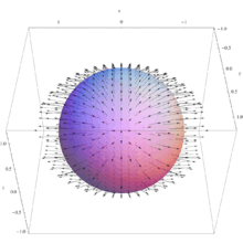
Suppose we wish to evaluate

where S is the unit sphere defined by

and F is the vector field

The direct computation of this integral is quite difficult, but we can simplify the derivation of the result using the divergence theorem, because the divergence theorem says that the integral is equal to:

where W is the unit ball:

Since the function y is positive in one hemisphere of W and negative in the other, in an equal and opposite way, its total integral over W is zero. The same is true for z:

Therefore,

because the unit ball W has volume 4π/3.
Applications
Differential form and integral form of physical laws
As a result of the divergence theorem, a host of physical laws can be written in both a differential form (where one quantity is the divergence of another) and an integral form (where the flux of one quantity through a closed surface is equal to another quantity). Three examples are Gauss's law (in electrostatics), Gauss's law for magnetism, and Gauss's law for gravity.
Continuity equations
Continuity equations offer more examples of laws with both differential and integral forms, related to each other by the divergence theorem. In fluid dynamics, electromagnetism, quantum mechanics, relativity theory, and a number of other fields, there are continuity equations that describe the conservation of mass, momentum, energy, probability, or other quantities. Generically, these equations state that the divergence of the flow of the conserved quantity is equal to the distribution of sources or sinks of that quantity. The divergence theorem states that any such continuity equation can be written in a differential form (in terms of a divergence) and an integral form (in terms of a flux).[8]
Inverse-square laws
Any inverse-square law can instead be written in a Gauss' law-type form (with a differential and integral form, as described above). Two examples are Gauss' law (in electrostatics), which follows from the inverse-square Coulomb's law, and Gauss' law for gravity, which follows from the inverse-square Newton's law of universal gravitation. The derivation of the Gauss' law-type equation from the inverse-square formulation (or vice versa) is exactly the same in both cases; see either of those articles for details.[8]
History
The theorem was first discovered by Lagrange in 1762,[9] then later independently rediscovered by Gauss in 1813,[10] by Ostrogradsky, who also gave the first proof of the general theorem, in 1826,[11] by Green in 1828,[12] etc.[13] Subsequently, variations on the divergence theorem are correctly called Ostrogradsky's theorem, but also commonly Gauss's theorem, or Green's theorem.
Examples
To verify the planar variant of the divergence theorem for a region R:

and the vector field:

The boundary of R is the unit circle, C, that can be represented parametrically by:

such that 0 ≤ s ≤ 2π where s units is the length arc from the point s = 0 to the point P on C. Then a vector equation of C is

At a point P on C:

Therefore,

Because M = 2y, ∂M/∂x = 0, and because N = 5x, ∂N/∂y = 0. Thus

Generalizations
Multiple dimensions
One can use the general Stokes' Theorem to equate the n-dimensional volume integral of the divergence of a vector field F over a region U to the (n − 1)-dimensional surface integral of F over the boundary of U:

This equation is also known as the Divergence theorem.
When n = 2, this is equivalent to Green's theorem.
When n = 1, it reduces to the Fundamental theorem of calculus.
Tensor fields
Writing the theorem in Einstein notation:


suggestively, replacing the vector field F with a rank-n tensor field T, this can be generalized to:[14]


where on each side, tensor contraction occurs for at least one index. This form of the theorem is still in 3d, each index takes values 1, 2, and 3. It can be generalized further still to higher (or lower) dimensions (for example to 4d spacetime in general relativity[15]).
See also
Notes
- ↑ or less correctly as Gauss' theorem (see history for reason)
- ↑ Katz, Victor J. (1979). "The history of Stokes's theorem". Mathematics Magazine. Mathematical Association of America. 52: 146–156. doi:10.2307/2690275. reprinted in Anderson, Marlow (2009). Who Gave You the Epsilon?: And Other Tales of Mathematical History. Mathematical Association of America. pp. 78–79. ISBN 0883855690.
- ↑ Stewart, James (2008), "Vector Calculus", Calculus: Early Transcendentals (6 ed.), Thomson Brooks/Cole, ISBN 978-0-495-01166-8
- ↑ R. G. Lerner; G. L. Trigg (1994). Encyclopaedia of Physics (2nd ed.). VHC. ISBN 3-527-26954-1.
- ↑ Byron, Frederick; Fuller, Robert (1992), Mathematics of Classical and Quantum Physics, Dover Publications, p. 22, ISBN 978-0-486-67164-2
- 1 2 M. R. Spiegel; S. Lipschutz; D. Spellman (2009). Vector Analysis. Schaum’s Outlines (2nd ed.). USA: McGraw Hill. ISBN 978-0-07-161545-7.
- 1 2 MathWorld
- 1 2 C.B. Parker (1994). McGraw Hill Encyclopaedia of Physics (2nd ed.). McGraw Hill. ISBN 0-07-051400-3.
- ↑ In his 1762 paper on sound, Lagrange treats a special case of the divergence theorem: Lagrange (1762) "Nouvelles recherches sur la nature et la propagation du son" (New researches on the nature and propagation of sound), Miscellanea Taurinensia (also known as: Mélanges de Turin ), 2: 11 - 172. This article is reprinted as: "Nouvelles recherches sur la nature et la propagation du son" in: J.A. Serret, ed., Oeuvres de Lagrange, (Paris, France: Gauthier-Villars, 1867), vol. 1, pages 151-316; on pages 263-265, Lagrange transforms triple integrals into double integrals using integration by parts.
- ↑ C. F. Gauss (1813) "Theoria attractionis corporum sphaeroidicorum ellipticorum homogeneorum methodo nova tractata," Commentationes societatis regiae scientiarium Gottingensis recentiores, 2: 355-378; Gauss considered a special case of the theorem; see the 4th, 5th, and 6th pages of his article.
- ↑ Mikhail Ostragradsky presented his proof of the divergence theorem to the Paris Academy in 1826; however, his work was not published by the Academy. He returned to St. Petersburg, Russia, where in 1828-1829 he read the work that he'd done in France, to the St. Petersburg Academy, which published his work in abbreviated form in 1831.
- His proof of the divergence theorem -- "Démonstration d'un théorème du calcul intégral" (Proof of a theorem in integral calculus) -- which he had read to the Paris Academy on February 13, 1826, was translated, in 1965, into Russian together with another article by him. See: Юшкевич А.П. (Yushkevich A.P.) and Антропова В.И. (Antropov V.I.) (1965) "Неопубликованные работы М.В. Остроградского" (Unpublished works of MV Ostrogradskii), Историко-математические исследования (Istoriko-Matematicheskie Issledovaniya / Historical-Mathematical Studies), 16: 49-96; see the section titled: "Остроградский М.В. Доказательство одной теоремы интегрального исчисления" (Ostrogradskii M. V. Dokazatelstvo odnoy teoremy integralnogo ischislenia / Ostragradsky M.V. Proof of a theorem in integral calculus).
- M. Ostrogradsky (presented: November 5, 1828 ; published: 1831) "Première note sur la théorie de la chaleur" (First note on the theory of heat) Mémoires de l'Académie impériale des sciences de St. Pétersbourg, series 6, 1: 129-133; for an abbreviated version of his proof of the divergence theorem, see pages 130-131.
- Victor J. Katz (May1979) "The history of Stokes' theorem," Mathematics Magazine, 52(3): 146-156; for Ostragradsky's proof of the divergence theorem, see pages 147-148.
- ↑ George Green, An Essay on the Application of Mathematical Analysis to the Theories of Electricity and Magnetism (Nottingham, England: T. Wheelhouse, 1838). A form of the "divergence theorem" appears on pages 10-12.
- ↑ Other early investigators who used some form of the divergence theorem include:
- Poisson (presented: February 2, 1824 ; published: 1826) "Mémoire sur la théorie du magnétisme" (Memoir on the theory of magnetism), Mémoires de l'Académie des sciences de l'Institut de France, 5: 247-338; on pages 294-296, Poisson transforms a volume integral (which is used to evaluate a quantity Q) into a surface integral. To make this transformation, Poisson follows the same procedure that is used to prove the divergence theorem.
- Frédéric Sarrus (1828) "Mémoire sur les oscillations des corps flottans" (Memoir on the oscillations of floating bodies), Annales de mathématiques pures et appliquées (Nismes), 19: 185-211.
- ↑ K.F. Riley; M.P. Hobson; S.J. Bence (2010). Mathematical methods for physics and engineering. Cambridge University Press. ISBN 978-0-521-86153-3.
- ↑ see for example:
J.A. Wheeler; C. Misner; K.S. Thorne (1973). Gravitation. W.H. Freeman & Co. pp. 85–86, §3.5. ISBN 0-7167-0344-0., and
R. Penrose (2007). The Road to Reality. Vintage books. ISBN 0-679-77631-1.
External links
- Hazewinkel, Michiel, ed. (2001), "Ostrogradski formula", Encyclopedia of Mathematics, Springer, ISBN 978-1-55608-010-4
- Differential Operators and the Divergence Theorem at MathPages
- The Divergence (Gauss) Theorem by Nick Bykov, Wolfram Demonstrations Project.
- Weisstein, Eric W. "Divergence Theorem". MathWorld.
— This article was originally based on the GFDL article from PlanetMath at http://planetmath.org/encyclopedia/Divergence.html