Finite volume method for two dimensional diffusion problem
The methods used for solving two dimensional Diffusion problems are similar to those used for one dimensional problems. The general equation for steady diffusion can be easily derived from the general transport equation for property Φ by deleting transient and convective terms[1]

where,
is the Diffusion coefficient[2] and is the Source term.[3]


A portion of the two dimensional grid used for Discretization is shown below:
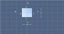
In addition to the east (E) and west (W) neighbors, a general grid node P , now also has north (N) and south (S) neighbors. The same notation is used here for all faces and cell dimensions as in one dimensional analysis. When the above equation is formally integrated over the Control volume, we obtain

Using the divergence theorem, the equation can be rewritten as :
![\left[{\Gamma{}}_eA_e\left(\frac{\partial{}\phi{}}{\partial{}x}\right)_{e}-{\Gamma{}}_wA_w\left(\frac{\partial{}\phi{}}{\partial{}x}\right)_{w}\right]+\left[{\Gamma{}}_nA_n\left(\frac{\partial{}\phi{}}{\partial{}y}\right)_{n}-{\Gamma{}}_sA_s\left(\frac{\partial{}\phi{}}{\partial{}y}\right)_{s}\right]+\bar{S}\Delta{}V=0](../I/m/7a48a35f6249079da78820a4cdd4373eeb7e2693.svg)
This equation represents the balance of generation of the property φ in a Control volume and the fluxes through its cell faces. The derivatives can by represented as follows by using Taylor series approximation:

Flux across the east face =

Flux across the south face =

Flux across the north face =

Substituting these expressions in equation (2) we obtain

When the source term is represented in linearized form , this equation can be rearranged as,

=
![\left[
\frac{{\Gamma{}}_eA_e}{{\delta{}x}_{PE}}
+ \frac{{\Gamma{}}_wA_w}{{\delta{}x}_{WP}}
+ \frac{{\Gamma{}}_nA_n}{{\delta{}y}_{PN}}
+ \frac{{\Gamma{}}_sA_s}{{\delta{}y}_{SP}}
- S_p\right] \phi{}_P](../I/m/9ac6a289ab2581a71e4a4e2606a5aebfecb315fe.svg)

This equation can now be expressed in a general discretized equation form for internal nodes, i.e.,

Where,


The face areas in y two dimensional case are :

and
.

We obtain the distribution of the property i.e. a given two dimensional situation by writing discretized equations of the form of equation (3) at each grid node of the subdivided domain. At the boundaries where the temperature or fluxes are known the discretized equation are modified to incorporate the boundary conditions. The boundary side coefficient is set to zero (cutting the link with the boundary) and the flux crossing this boundary is introduced as a source which is appended to any existing and terms. Subsequently the resulting set of equations is solved to obtain the two dimensional distribution of the property


References
- Patankar, Suhas V. (1980), Numerical Heat Transfer and Fluid Flow, Hemisphere.
- Hirsch, C. (1990), Numerical Computation of Internal and External Flows, Volume 2: Computational Methods for Inviscid and Viscous Flows, Wiley.
- Laney, Culbert B.(1998), Computational Gas Dynamics, Cambridge University Press.
- LeVeque, Randall(1990), Numerical Methods for Conservation Laws, ETH Lectures in Mathematics Series, Birkhauser-Verlag.
- Tannehill, John C., et al., (1997), Computational Fluid mechanics and Heat Transfer, 2nd Ed., Taylor and Francis.
- Wesseling, Pieter(2001), Principles of Computational Fluid Dynamics, Springer-Verlag.
- Carslaw, H. S. and Jager, J. C. (1959). Conduction of Heat in Solids. Oxford: Clarendon Press
- Crank, J. (1956). The Mathematics of Diffusion. Oxford: Clarendon Press
- Thambynayagam, R. K. M (2011). The Diffusion Handbook: Applied Solutions for Engineers: McGraw-Hill
- ↑ "Navier-Stokes Equations in Fluid Mechanics". Efunda.com. Retrieved 2013-10-29.
- ↑ "Diffusion – useful equations". Life.illinois.edu. Retrieved 2013-10-29.
- ↑ "SSCP: Programming Strategies". Physics.drexel.edu. Retrieved 2013-10-29.
External links
- http://opencourses.emu.edu.tr/course/view.php?id=27&lang=en
- http://www.nptel.iitm.ac.in/courses/112105045/
- http://ingforum.haninge.kth.se/armin/CFD/dirCFD.htm
- Diffusion equation
- Computational fluid dynamics
- Convection–diffusion equation
- Finite volume method, Cheng Long
- Finite volume method, Robert Eymard et al. (2010), Scholarpedia,5(6):9835
See also
- Computational fluid dynamics
- Finite difference
- Heat equation
- Fokker-Planck equation
- Fick's law of diffusion: Fick's Second Law
- Maxwell-Stefan equation
- Diffusion equation