File dynamics

The term file dynamics is the motion of many particles in a narrow channel.

In science: in chemistry, physics, mathematics and related fields, file dynamics (sometimes called, single file dynamics) is the diffusion of N (N → ∞) identical Brownian hard spheres in a quasi-one-dimensional channel of length L (L → ∞), such that the spheres do not jump one on top of the other, and the average particle's density is approximately fixed. The most famous statistical properties of this process is that the mean squared displacement (MSD) of a particle in the file follows, $\mathrm {MSD} \approx t^{\frac {1}{2}}$ , and its probability density function (PDF) is Gaussian in position with a variance MSD.^[1]^[2]^[3]

Results in files that generalize the basic file include:

In files with a density law that is not fixed, but decays as a power law with an exponent a with the distance from the origin, the particle in the origin has a MSD that scales like, $MSD\approx t^{\frac {1+a}{2}}$ , with a Gaussian PDF.^[4]
When, in addition, the particles' diffusion coefficients are distributed like a power law with exponent γ (around the origin), the MSD follows, $MSD\approx t^{\frac {1-\gamma }{2/(1+a)-\gamma }}$ , with a Gaussian PDF.^[5]
In anomalous files that are renewal, namely, when all particles attempt a jump together, yet, with jumping times taken from a distribution that decays as a power law with an exponent, −1 − α, the MSD scales like the MSD of the corresponding normal file, in the power of α.^[6]
In anomalous files of independent particles, the MSD is very slow and scales like, $MSD\approx log^{2}(t)$ . Even more exciting, the particles form clusters in such files, defining a dynamical phase transition. This depends on the anomaly power α: the percentage of particles in clusters ξ follows, $\xi \approx {\sqrt {1-\alpha ^{3}}}$ .^[7]
Other generalizations include: when the particles can bypass each other with a constant probability upon encounter, an enhanced diffusion is seen.^[8] When the particles interact with the channel, a slower diffusion is observed.^[9] Files in embedded in two-dimensions show similar characteristics of files in one dimension.^[7]

Generalizations of the basic file are important since these models represent reality much more accurately than the basic file. Indeed, file dynamics are used in modeling numerous microscopic processes:^[10]^[11]^[12]^[13]^[14]^[15]^[16] the diffusion within biological and synthetic pores and porous material, the diffusion along 1D objects, such as in biological roads, the dynamics of a monomer in a polymer, etc.

Mathematical formulation

Simple files

In simple Brownian files, $P(\mathbf {x} ,t\mid \mathbf {x_{0}} )$ , the joint probability density function (PDF) for all the particles in file, obeys a normal diffusion equation:

$\partial _{t}P(\mathbf {x} ,t\mid \mathbf {x_{0}} )=D\Sigma _{j=-M}^{M}\partial _{x_{j}}^{2}P(\mathbf {x} ,t\mid \mathbf {x_{0}} ).$

(1)

In $P(\mathbf {x} ,t\mid \mathbf {x_{0}} )$ , $\mathbf {x} =\{x_{-M},x_{-M+1},\ldots ,x_{M}\}$ is the set of particles' positions at time $t$ and $\mathbf {x_{0}}$ is the set of the particles' initial positions at the initial time $t_{0}$ (set to zero). Equation (1) is solved with the appropriate boundary conditions, which reflect the hard-sphere nature of the file:

${\big (}D\partial _{x_{j}}P(\mathbf {x} ,t\mid \mathbf {x_{0}} ){\big )}_{x_{j}=x_{j+1}}={\big (}D\partial _{x_{j+1}}P(\mathbf {x} ,t\mid \mathbf {x_{0}} ){\big )}_{x_{j+1}=x_{j}};\qquad j=-M,\ldots ,M-1,$

(2)

and with the appropriate initial condition:

$P(\mathbf {x} ,t\rightarrow \infty \mid x_{0})=\Pi _{j=-M}^{M}\delta (x_{j}-x_{0,j}).$

(3)

In a simple file, the initial density is fixed, namely, $x_{0,j}=j\Delta$ , where $\Delta$ is a parameter that represents a microscopic length. The PDFs' coordinates must obey the order: $x_{-M}\leq x_{-M+1}\leq \cdots \leq x_{M}$ .

Heterogeneous files

In such files, the equation of motion follows,

$\partial _{t}P(\mathbf {x} ,t\mid \mathbf {x_{0}} )=\Sigma _{j=-M}^{M}D_{j}\partial _{x_{j}}^{2}P(\mathbf {x} ,t\mid \mathbf {x_{0}} ).$

(4)

with the boundary conditions:

${\big (}D_{j}\partial _{x_{j}}P(\mathbf {x} ,t\mid \mathbf {x_{0}} ){\big )}_{x_{j}=x_{j+1}}={\big (}D_{j+1}\partial _{x_{j+1}}P(\mathbf {x} ,t\mid \mathbf {x_{0}} ){\big )}_{x_{j+1}=x_{j}};\qquad j=-M,\ldots ,M-1,$

(5)

and with the initial condition, Eq. (3), where the particles’ initial positions obey:

$x0,j=sign(j)\Delta \mid j\mid ^{1/(1-a)};\qquad 0\leq {\mathit {a}}\leq 1.$

(6)

The file diffusion coefficients are taken independently from the PDF,

$W(D)={\frac {1-\gamma }{\Lambda }}(D/\Lambda )^{-\gamma },\qquad 0\leq \gamma \leq 1,$

(7)

where Λ has a finite value that represents the fastest diffusion coefficient in the file.

Renewal, anomalous, heterogeneous files

In renewal-anomalous files, a random period is taken independently from a waiting time probability density function (WT-PDF; see Continuous-time Markov process for more information) of the form: $\psi _{\alpha }(t)\sim k(kt)^{-1-\alpha },0<\alpha \leq 1$ , where k is a parameter. Then, all the particles in the file stand still for this random period, where afterwards, all the particles attempt jumping in accordance with the rules of the file. This procedure is carried on over and over again. The equation of motion for the particles’ PDF in a renewal-anomalous file is obtained when convoluting the equation of motion for a Brownian file with a kernel $k_{\alpha }(t)$ :

$\partial _{t}P(\mathbf {x} ,t\mid \mathbf {x_{0}} )=\Sigma _{j=-M}^{M}D_{j}\partial _{x_{j}}^{2}\int _{0}^{t}k_{\alpha }(t-u)P(\mathbf {x} ,u\mid \mathbf {x_{0}} )\,du.$

(8)

Here, the kernel $k_{\alpha }(t)$ and the WT-PDF $\psi _{\alpha }(t)$ are related in Laplace space, ${\bar {k}}_{\alpha }(s)={\frac {s{\bar {\psi }}_{\alpha }(s)}{1-{\bar {\psi }}_{\alpha }(s)}}$ . (The Laplace transform of a function $f(t)$ reads, ${\bar {f}}(s)=\int _{0}^{\infty }f(t)e^{-st}\,dt$ .) The reflecting boundary conditions accompanied Eq. (8) are obtained when convoluting the boundary conditions of a Brownian file with the kernel $k_{\alpha }(t)$ , where here and in a Brownian file the initial conditions are identical.

Anomalous files with independent particles

When each particle in the anomalous file is assigned with its own jumping time drawn form $\psi _{\alpha }(t)$ ( $\psi _{\alpha }(t)$ is the same for all the particles), the anomalous file is not a renewal file. The basic dynamical cycle in such a file consists of the following steps: a particle with the fastest jumping time in the file, say, $t_{i}$ for particle i, attempts a jump. Then, the waiting times for all the other particles are adjusted: we subtract $t_{i}$ from each of them. Finally, a new waiting time is drawn for particle i. The most crucial difference among renewal anomalous files and anomalous files that are not renewal is that when each particle has its own clock, the particles are in fact connected also in the time domain, and the outcome is further slowness in the system (proved in the main text). The equation of motion for the PDF in anomalous files of independent particles reads:

$\partial _{t_{i}}P(\mathbf {x} ,\mathbf {t} \mid \mathbf {x_{0}} )=D_{i}\partial _{x_{i}}^{2}\int _{0}^{t_{i}}k_{\alpha }(t_{i}-u_{i})P(\mathbf {x} ,\mathbf {t} ^{'(i)},u_{i}\mid \mathbf {x_{0}} )\,du_{i};\qquad -M\leq i\leq M.$

(9)

Note that the time argument in the PDF $P(\mathbf {x} ,\mathbf {t} \mid \mathbf {x_{0}} )$ is a vector of times: $\mathbf {t} =\{t_{i}\}_{i=-M}^{M}$ , and $\mathbf {t} ^{'(i)}=\{t_{c}\}_{c=-M,c\neq i}^{M}$ . Adding all the coordinates and performing the integration in the order of faster times first (the order is determined randomly from a uniform distribution in the space of configurations) gives the full equation of motion in anomalous files of independent particles (averaging of the equation over all configurations is therefore further required). Indeed, even Eq. (9) is very complicated, and averaging further complicates things.

Mathematical analysis

Simple files

The solution of Eqs. (1)-(2) is a complete set of permutations of all initial coordinates appearing in the Gaussians,^[4]

$P(\mathbf {x} ,\mid \mathbf {x_{0}} )={\frac {1}{c_{N}}}\Sigma _{\{p\}}e^{-1/4Dt\Sigma _{j=-M}^{M}(x_{j}-x_{0,j}(p))^{2}}.$

(10)

Here, the index $p$ goes on all the permutations of the initial coordinates, and contains $N!$ permutations. From Eq. (10), the PDF of a tagged particle in the file, $P(r,t\mid r_{0})$ , is calculated ^[4]

$P(r,t\mid r_{0})\sim {\frac {1}{c_{N}}}e^{-R_{d}^{2}/{\sqrt {2\tau }}},$

(11)

In Eq. (11), $R_{d}=r_{d}\Delta$ , $r_{d}=r-r_{0}$ ( $r_{0}$ is the initial condition of the tagged particle), and $\tau =\Delta ^{-2}Dt$ . The MSD for the tagged particle is obtained directly from Eq. (11):

$\langle R_{d}^{2}\rangle \sim {\sqrt {\tau }}.$

(12)

Heterogeneous files

The solution of Eqs. (4)-(7) is approximated with the expression,^[5]

$P(x,t\mid x_{0})\approx {\frac {1}{c_{N}}}\Sigma _{\{p\}}e^{-\Sigma _{j=-M}^{M}(x_{j}-x_{0,j}(p))^{2}/4tD_{j}}.$

(13)

Starting from Eq. (13), the PDF of the tagged particle in the heterogeneous file follows,^[5]

$P(r,t\mid r_{0})\sim {\frac {1}{c_{N}}}e^{-R_{d}^{2}/4\tau \tau ^{(1-a))/(2-\gamma (1+a))}};\qquad \tau =\Delta ^{-2}\Lambda t.$

(14)

The MSD of a tagged particle in a heterogeneous file is taken from Eq. (14):

$\langle R_{d}^{2}\rangle =2\tau ^{(1-\gamma )/(2c-\gamma )},\qquad c=1/((1+a)).$

(15)

Renewal anomalous heterogeneous files

The results of renewal-anomalous files are simply derived from the results of Brownian files. Firstly, the PDF in Eq. (8) is written in terms of the PDF that solves the un-convoluted equation, that is, the Brownian file equation; this relation is made in Laplace space:

${\bar {P}}(x,s\mid x_{0})={\frac {1}{{\bar {k}}_{\alpha }(s)}}{\bar {P}}_{\text{nrml}}(x,s/{\bar {k}}_{\alpha }(s)\mid x_{0}).$

(16)

(The subscript nrml stands for normal dynamics.) From Eq. (16), it is straightforward relating the MSD of Brownian heterogeneous files and renewal-anomalous heterogeneous files,^[6]

$\langle {\bar {r}}^{2}(s)\rangle ={\frac {1}{{\bar {k}}_{\alpha }(s)}}\langle {\bar {r}}^{2}(s/{\bar {k}}_{\alpha }(s))\rangle _{\text{nrml}}.$

(17)

From Eq. (18), one finds that the MSD of a file with normal dynamics in the power of $\alpha$ is the MSD of the corresponding renewal-anomalous file,^[6]

$\langle r^{2}(t)\rangle \sim \langle r^{2}(t)\rangle _{\text{nrml}}^{\alpha }.$

(19)

Anomalous files with independent particles

The equation of motion for anomalous files with independent particles, (9), is very complicated. Solutions for such files are reached while deriving scaling laws and with numerical simulations.

Scaling laws for anomalous files of independent particles

Firstly, we write down the scaling law for the mean absolute displacement (MAD) in a renewal file with a constant density:^[4]^[5]^[7]

$\langle \mid r\mid \rangle \sim \langle \mid r\mid \rangle _{\text{free}}/n.$

(20)

Here, $n$ is the number of particles in the covered-length $\langle \mid r\mid \rangle$ , and $\langle \mid r\mid \rangle _{\text{free}}$ is the MAD of a free anomalous particle, $\langle \mid r\mid \rangle _{\text{free}}\sim t^{\alpha /2})$ . In Eq. (20), $n$ enters the calculations since all the particles within the distance $\langle \mid r\mid \rangle$ from the tagged one must move in the same direction in order that the tagged particle will reach a distance $\langle \mid r\mid \rangle$ from its initial position. Based on Eq. (20), we write a generalized scaling law for anomalous files of independent particles:

$\langle |r|\rangle \sim {\frac {\langle \mid r\mid \rangle _{\text{free}}}{n}}f(n);\qquad 0<f(n)<1.$

(21)

The first term on the right hand side of Eq. (21) appears also in renewal files; yet, the term f(n) is unique. f(n) is the probability that accounts for the fact that for moving n anomalous independent particles in the same direction, when these particles indeed try jumping in the same direction (expressed with the term, ( $\langle \mid r\mid \rangle _{\text{free}}/n)$ ), the particles in the periphery must move first so that the particles in the middle of the file will have the free space for moving, demanding faster jumping times for those in the periphery. f(n) appears since there is not a typical timescale for a jump in anomalous files, and the particles are independent, and so a particular particle can stand still for a very long time, substantially limiting the options of progress for the particles around him, during this time. Clearly, $0<f(n)<1$ , where f(n) = 1 for renewal files since the particles jump together, yet also in files of independent particles with $\alpha >1$ , since in such files there is a typical timescale for a jump, considered the time for a synchronized jump. We calculate f(n) from the number of configurations in which the order of the particles’ jumping times enables motion; that is, an order where the faster particles are always located towards the periphery. For n particles, there are n! different configurations, where one configuration is the optimal one; so, $(1/n!)\leq f(n)$ . Yet, although not optimal, propagation is also possible in many other configurations; when m is the number of particles that move, then,

$f(n)\sim {\dbinom {n}{m}}(n-m)!1/n!,$

(22)

where ${\dbinom {n}{m}}(n-m)!$ counts the number of configurations in which those m particles around the tagged one have the optimal jumping order. Now, even when m~n/2, $f(n)\sim e^{-n/2}$ . Using in Eq. (21), $f(n)\sim e^{-n/n_{0}}$ ( $n_{0}$ a small number larger than 1), we see,

$\mathrm {MSD} \sim \left({\frac {\alpha }{n_{0}}}\right)^{2}\ln ^{2}(t).$

(23)

(In Eq. (23), we use, $MSD\sim \mid MAD\mid ^{2}$ .) Equation (23) shows that asymptotically the particles are extremely slow in anomalous files of independent particles.

Numerical studies of anomalous files of independent particles

Figure 1 Trajectories from simulations of 501 anomalous, independent, particles, with

\alpha =0.9,0.1

(recommended: open the file in a new window)

With numerical studies, one sees that anomalous files of independent particles form clusters. This phenomenon defines a dynamical phase transition. At steady state, the percentage of particles in cluster, $\xi (\alpha )$ , follows,

$\xi (\alpha )\approx {\sqrt {1-\alpha ^{3}}}$

(24)

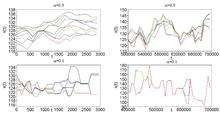
In Figure 1 we show trajectories from 9 particles in a file of 501 particles. (It is recommended opening the file in a new window). The upper panels show trajetcories for $\alpha =0.9$ and the lower panels show trajectories for $\alpha=0.1$ . For each value of $\alpha$ shown are trajectories in the early stages of the simulations (left) and in all stages of the simulation (right). The panels exhibit the phenomenon of the clustering, where the trajectories attract each other and then move pretty much together.

References

↑ Harris T. E. (1965) "Diffusion with 'Collisions' between Particles", Journal of Applied Probability, 2 (2), 323-338 JSTOR 3212197
↑ Jepsen D. W., J. Math. Phys. (N.Y.), 6 (1965) 405.
↑ Lebowitz J. L., Percus J. K., Phys. Rev., 155 (1967) 122.
1 2 3 4 Flomenbom O. and Taloni A., Europhys. Lett., 83 (2008) 20004.
1 2 3 4 Flomenbom O., Phys. Rev. E, 82 (2010) 031126.
1 2 3 Flomenbom O., Phys. Lett. A, 374 (2010) 4331.
1 2 3 Flomenbom O., EPL 94, 58001 (2011).
↑ Mon K. K. and Percus J. K., J. Chem. Phys., 117 (2002) 2289.
↑ Taloni A. and Marchesoni F., Phys. Rev. Lett., 96 (2006) 020601.
↑ Kärger J. and Ruthven D. M. (1992) Diffusion in Zeolites and Other Microscopic Solids (Wiley, NY).
↑ Wei Q. H., Bechinger C. and Leiderer P., Science, 287 (2000) 625.
↑ de Gennes J. P., J. Chem. Phys., 55 (1971) 572.
↑ Richards P. M., Phys. Rev. B, 16 (1977) 1393.
↑ Maxfield F. R., Curr. Opin. Cell Biol., 14 (2002) 483.
↑ Biological Membrane Ion Channels: Dynamics, Structure, And Applications, Chung S-h., Anderson O. S. and Krishnamurthy V. V., editors (Springer-verlag) 2006.
↑ Howard J., Mechanics of Motor Proteins and the Cytoskeleton (Sinauer associates Inc. Sunderland, MA) 2001.

This article is issued from Wikipedia - version of the 11/8/2013. The text is available under the Creative Commons Attribution/Share Alike but additional terms may apply for the media files.

File dynamics

Mathematical formulation

Simple files

Heterogeneous files

Renewal, anomalous, heterogeneous files

Anomalous files with independent particles

Mathematical analysis

Simple files

Heterogeneous files

Renewal anomalous heterogeneous files

Anomalous files with independent particles

Scaling laws for anomalous files of independent particles

Numerical studies of anomalous files of independent particles

See also

References