Fidelity of quantum states
In quantum information theory, fidelity is a measure of the "closeness" of two quantum states. It is not a metric on the space of density matrices, but it can be used to define the Bures metric on this space.
Motivation
Given two random variables X, Y with values (1...n) and probabilities p = (p1...pn) and q = (q1...qn). The fidelity of X and Y is defined to be the quantity
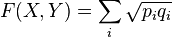 .
.
The fidelity deals with the marginal distribution of the random variables. It says nothing about the joint distribution of those variables. In other words, the fidelity F(X,Y) is the inner product of  and
and  viewed as vectors in Euclidean space. Notice that F(X,Y) = 1 if and only if p = q. In general,
  . This measure is known as the Bhattacharyya coefficient.
Given a classical measure of the distinguishability of two probability distributions, one can motivate a measure of distinguishability of two quantum states as follows. If an experimenter is attempting to determine whether a quantum state is either of two possibilities  or
or  , the most general possible measurement they can make on the state is a POVM, which is described by a set of Hermitian positive semidefinite operators
  . If the state given to the experimenter is , they will witness outcome
  with probability
 ![p_i = \mathrm{Tr}[ \rho F_i ]](../I/m/b7caeb768da25b587395656b8f1b3012.png) , and likewise with probability
, and likewise with probability ![q_i = \mathrm{Tr}[ \sigma F_i ]](../I/m/f054d4f1ce940e152d80a659ffb1b057.png) for . Their ability to distinguish between the quantum states and is then equivalent to their ability to distinguish between the classical probability distributions
for . Their ability to distinguish between the quantum states and is then equivalent to their ability to distinguish between the classical probability distributions  and
and  . Naturally, the experimenter will choose the best POVM he can find, so this motivates defining the quantum fidelity as the Bhattacharyya coefficient when extremized over all possible POVMs :
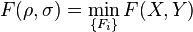 .
.
![= \min_{\{F_i\}} \sum _i \sqrt{\mathrm{Tr}[ \rho F_i ] \mathrm{Tr}[ \sigma F_i ]}](../I/m/6923468d7272ad25d2bea7e221f81861.png) .
.
It was shown by Fuchs and Caves that this manifestly symmetric definition is equivalent to the simple asymmetric formula given in the next section.[1]
Definition
Given two density matrices ρ and σ, the fidelity is defined by
![F(\rho, \sigma) = \operatorname{Tr} \left[\sqrt{\sqrt{\rho} \sigma \sqrt{\rho}}\right].](../I/m/edaf414aad5daba2cb8bf8799b00971b.png)
By M½ of a positive semidefinite matrix M, we mean its unique positive square root given by the spectral theorem. The Euclidean inner product from the classical definition is replaced by the Hilbert–Schmidt inner product. When the states are classical, i.e. when ρ and σ commute, the definition coincides with that for probability distributions.
An equivalent definition is given by
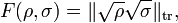
where the norm is the trace norm (sum of the singular values). This definition has the advantage that it clearly shows that the fidelity is symmetric in its two arguments.
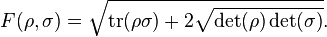
For two qubit states and it can be shown that the fidelity can be calculated as
Notice by definition F is non-negative, and F(ρ,ρ) = 1. In the following section it will be shown that it can be no larger than 1.
In the original 1994 paper of Jozsa the name 'fidelity' was used for the quantity
 and this convention is often used in the literature.
According to this convention 'fidelity' has a meaning of probability.
and this convention is often used in the literature.
According to this convention 'fidelity' has a meaning of probability.
Simple examples
Pure states
Suppose that one of the states is pure:  . Then
  and the fidelity is
![F(\rho, \sigma) = \operatorname{Tr} \left[\sqrt{ | \phi \rangle \langle \phi | \sigma | \phi \rangle \langle \phi |} \right]
= \sqrt{\langle \phi | \sigma | \phi \rangle} \operatorname{Tr} \left[\sqrt{ | \phi \rangle \langle \phi |} \right]
= \sqrt{\langle \phi | \sigma | \phi \rangle}.](../I/m/cfd13e2d26f9b16f9ca240f069598823.png)
If the other state is also pure,  , then the fidelity is
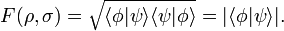
This is sometimes called the overlap between two states. If, say,  is an eigenstate of an observable, and the system is prepared in
  , then F(ρ, σ)2 is the probability of the system being in state after the measurement.
Commuting states
Let ρ and σ be two density matrices that commute. Therefore they can be simultaneously diagonalized by unitary matrices, and we can write
 and
and 
for some orthonormal basis  . Direct calculation shows the fidelity is

This shows that, heuristically, fidelity of quantum states is a genuine extension of the notion from probability theory.
Some properties
Unitary invariance
Direct calculation shows that the fidelity is preserved by unitary evolution, i.e.

for any unitary operator U.
Uhlmann's theorem
We saw that for two pure states, their fidelity coincides with the overlap. Uhlmann's theorem generalizes this statement to mixed states, in terms of their purifications:
Theorem Let ρ and σ be density matrices acting on Cn. Let ρ½ be the unique positive square root of ρ and

be a purification of ρ (therefore  is an orthonormal basis), then the following equality holds:

where  is a purification of σ. Therefore, in general, the fidelity is the maximum overlap between purifications.
Proof:
A simple proof can be sketched as follows. Let  denote the vector

and σ½ be the unique positive square root of σ. We see that, due to the unitary freedom in square root factorizations and choosing orthonormal bases, an arbitrary purification of σ is of the form

where Vi's are unitary operators. Now we directly calculate

But in general, for any square matrix A and unitary U, it is true that |Tr(AU)| ≤ Tr ((A*A)½). Furthermore, equality is achieved if U* is the unitary operator in the polar decomposition of A. From this follows directly Uhlmann's theorem.
Consequences
Some immediate consequences of Uhlmann's theorem are
- Fidelity is symmetric in its arguments, i.e. F (ρ,σ) = F (σ,ρ). Notice this is not obvious from the definition.
- F (ρ,σ) lies in [0,1], by the Cauchy–Schwarz inequality.
- F (ρ,σ) = 1 if and only if ρ = σ, since Ψρ = Ψσ implies ρ = σ.
So we can see that fidelity behaves almost like a metric. This can be formalised and made useful by defining

As the angle between the states and . It follows from the above properties that  is non-negative, symmetric in its inputs, and is equal to zero if and only if
  . Furthermore, it can be proved that it obeys the triangle inequality,[2] so this angle is a metric on the state space: the Fubini–Study metric.[3]
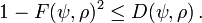
Relationship to trace distance
We can define the trace distance between two matrices A and B in terms of the trace norm by

When A and B are both density operators, this is a quantum generalization of the statistical distance. This is relevant because the trace distance provides upper and lower bounds on the fidelity as quantified by the Fuchs–van de Graaf inequalities,[4]

Often the trace distance is easier to calculate or bound than the fidelity, so these relationships are quite useful. In the case that at least one of the states is a pure state Ψ, the lower bound can be tightened.
References
- ↑ C. A. Fuchs, C. M. Caves: "Ensemble-Dependent Bounds for Accessible Information in Quantum Mechanics", Physical Review Letters 73, 3047(1994)
- ↑ M. Nielsen, I. Chuang, Quantum Computation and Quantum Information, Cambridge University Press, 2000, 409–416
- ↑ K. Życzkowski, I. Bengtsson, Geometry of Quantum States, Cambridge University Press, 2008, 131
- ↑ C. A. Fuchs and J. van de Graaf, "Cryptographic Distinguishability Measures for Quantum Mechanical States", IEEE Trans. Inf. Theory 45, 1216 (1999). arXiv:quant-ph/9712042
- A. Uhlmann "The "Transition Probability" in the State Space of a *-Algebra". Rep. Math. Phys. 9 (1976) 273–279. PDF
- R. Jozsa, "Fidelity for mixed quantum states", Journal of Modern Optics, 1994, vol. 41, 2315–2323.
- J. A. Miszczak, Z. Puchała, P. Horodecki, A. Uhlmann, K. Życzkowski, arXiv:0805.2037 "Sub- and super-fidelity as bounds for quantum fidelity", Quantum Information & Computation, Vol.9 No.1&2 (2009)