Electrical resistivity and conductivity
Electrical resistivity (also known as resistivity, specific electrical resistance, or volume resistivity) is an intrinsic property that quantifies how strongly a given material opposes the flow of electric current. A low resistivity indicates a material that readily allows the flow of electric current. Resistivity is commonly represented by the Greek letter ρ (rho). The SI unit of electrical resistivity is the ohm-metre (Ω⋅m).[1][2][3] As an example, if a 1 m × 1 m × 1 m solid cube of material has sheet contacts on two opposite faces, and the resistance between these contacts is 1 Ω, then the resistivity of the material is 1 Ω⋅m.
Electrical conductivity or specific conductance is the reciprocal of electrical resistivity, and measures a material's ability to conduct an electric current. It is commonly represented by the Greek letter σ (sigma), but κ (kappa) (especially in electrical engineering) or γ (gamma) are also occasionally used. Its SI unit is siemens per metre (S/m) and CGSE unit is reciprocal second (s−1).
Definition
Resistors or conductors with uniform cross-section
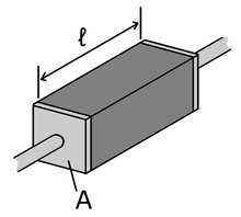
Many resistors and conductors have a uniform cross section with a uniform flow of electric current, and are made of one material. (See the adjacent diagram.) In this case, the electrical resistivity ρ (Greek: rho) is defined as:

where
- R is the electrical resistance of a uniform specimen of the material
- is the length of the piece of material
- A is the cross-sectional area of the specimen

The reason resistivity is defined this way is that it makes resistivity an intrinsic property, unlike resistance. All copper wires, irrespective of their shape and size, have approximately the same resistivity, but a long, thin copper wire has a much larger resistance than a thick, short copper wire. Every material has its own characteristic resistivity – for example, resistivity of rubber is far larger than copper's.
In a hydraulic analogy, passing current through a high-resistivity material is like pushing water through a pipe full of sand—while passing current through a low-resistivity material is like pushing water through an empty pipe. If the pipes are the same size and shape, the pipe full of sand has higher resistance to flow. Resistance, however, is not solely determined by the presence or absence of sand. It also depends on the length and width of the pipe: short or wide pipes have lower resistance than narrow or long pipes.
The above equation can be transposed to get Pouillet's law (named after Claude Pouillet):

The resistance of a given material increases with length, but decreases with increasing cross-sectional area. From the above equations, resistivity has SI units of ohm-metres (Ω·m).
The formula can be used to intuitively understand the meaning of a resistivity value. For example, if A = 1 m2 = 1 m (forming a cube with perfectly conductive contacts on opposite faces), then the resistance of this element in ohms is numerically equal to the resistivity of the material it is made of in Ω·m.

Conductivity, σ, is defined as the inverse of resistivity:

Conductivity has SI units of siemens per meter (S/m).
General definition
The above definition was specific to resistors or conductors with a uniform cross-section, where current flows uniformly through them. A more basic and general definition starts from the fact that an electric field inside a material makes electric current flow. The electrical resistivity, ρ, is defined as the ratio of the electric field to the density of the current it creates:

where
- ρ is the resistivity of the conductor material,
- E is the magnitude of the electric field,
- J is the magnitude of the current density,
in which E and J are inside the conductor.
Conductivity is the inverse:

For example, rubber is a material with large ρ and small σ—because even a very large electric field in rubber makes almost no current flow through it. On the other hand, copper is a material with small ρ and large σ—because even a small electric field pulls a lot of current through it.
Causes of conductivity
Band theory simplified

According to elementary quantum mechanics, electrons in an atom do not take on arbitrary energy values. Rather, electrons only occupy certain discrete energy levels in an atom or crystal; energies between these levels are impossible. When a large number of such allowed energy levels are spaced close together (in energy-space)—i.e. have similar (minutely differing) energies— we can talk about these energy levels together as an "energy band". There can be many such energy bands in a material, depending on the atomic number {number of electrons (if the atom is neutral)} and their distribution (besides external factors like environmental modification of the energy bands).
The material's electrons seek to minimize the total energy in the material by going to low energy states; however, the Pauli exclusion principle means that they cannot all go to the lowest state. The electrons instead "fill up" the band structure starting from the bottom. The characteristic energy level up to which the electrons have filled is called the Fermi level. The position of the Fermi level with respect to the band structure is very important for electrical conduction: only electrons in energy levels near the Fermi level are free to move around, since the electrons can easily jump among the partially occupied states in that region. In contrast, the low energy states are rigidly filled with a fixed number of electrons at all times, and the high energy states are empty of electrons at all times.
In metals there are many energy levels near the Fermi level, meaning that there are many electrons available to move. This is what causes the high electronic conductivity of metals.
An important part of band theory is that there may be forbidden bands in energy: energy intervals that contain no energy levels. In insulators and semiconductors, the number of electrons happens to be just the right amount to fill a certain integer number of low energy bands, exactly to the boundary. In this case, the Fermi level falls within a band gap. Since there are no available states near the Fermi level, and the electrons are not freely movable, the electronic conductivity is very low.
In metals
A metal consists of a lattice of atoms, each with an outer shell of electrons that freely dissociate from their parent atoms and travel through the lattice. This is also known as a positive ionic lattice.[4] This 'sea' of dissociable electrons allows the metal to conduct electric current. When an electrical potential difference (a voltage) is applied across the metal, the resulting electric field causes electrons to drift towards the positive terminal. The actual drift velocity of electrons is very small, in the order of magnitude of a meter per hour. However, as the electrons are densely packed in the material, the electromagnetic field is propagated through the metal at nearly the speed of light.[5] The mechanism is similar to transfer of momentum of balls in a Newton's cradle.[6]
Near room temperatures, metals have resistance. The primary cause of this resistance is the collision of electrons with the atoms that make up the crystal lattice. This acts to scatter electrons and lose their energy on collisions rather than on linear movement through the lattice. Also contributing to resistance in metals with impurities are the resulting imperfections in the lattice.[7]
The larger the cross-sectional area of the conductor, the more electrons per unit length are available to carry the current. As a result, the resistance is lower in larger cross-section conductors. The number of scattering events encountered by an electron passing through a material is proportional to the length of the conductor. The longer the conductor, therefore, the higher the resistance. Different materials also affect the resistance.[8]
In semiconductors and insulators
In metals, the Fermi level lies in the conduction band (see Band Theory, above) giving rise to free conduction electrons. However, in semiconductors the position of the Fermi level is within the band gap, approximately halfway between the conduction band minimum and valence band maximum for intrinsic (undoped) semiconductors. This means that at 0 kelvin, there are no free conduction electrons, and the resistance is infinite. However, the resistance continues to decrease as the charge carrier density in the conduction band increases. In extrinsic (doped) semiconductors, dopant atoms increase the majority charge carrier concentration by donating electrons to the conduction band or producing holes in the valence band. For both types of donor or acceptor atoms, increasing dopant density reduces resistance. Hence, highly doped semiconductors behave metallically. At very high temperatures, the contribution of thermally generated carriers dominate over the contribution from dopant atoms, and the resistance decreases exponentially with temperature.
In ionic liquids/electrolytes
In electrolytes, electrical conduction happens not by band electrons or holes, but by full atomic species (ions) traveling, each carrying an electrical charge. The resistivity of ionic solutions (electrolytes) varies tremendously with concentration – while distilled water is almost an insulator, salt water is a reasonable electrical conductor. Conduction in ionic liquids is also controlled by the movement of ions, but here we are talking about molten salts rather than solvated ions. In biological membranes, currents are carried by ionic salts. Small holes in cell membranes, called ion channels, are selective to specific ions and determine the membrane resistance.
Superconductivity
The electrical resistivity of a metallic conductor decreases gradually as temperature is lowered. In ordinary conductors, such as copper or silver, this decrease is limited by impurities and other defects. Even near absolute zero, a real sample of a normal conductor shows some resistance. In a superconductor, the resistance drops abruptly to zero when the material is cooled below its critical temperature. An electric current flowing in a loop of superconducting wire can persist indefinitely with no power source.[9]
In 1986, researchers discovered that some cuprate-perovskite ceramic materials have much higher critical temperatures, and in 1987 one was produced with a critical temperature above 90 K (−183 °C).[10] Such a high transition temperature is theoretically impossible for a conventional superconductor, so the researchers named these conductors high-temperature superconductors. Liquid nitrogen boils at 77 K, facilitating many experiments and applications that are less practical at lower temperatures. In conventional superconductors, electrons are held together in pairs by an attraction mediated by lattice phonons. The best available model of high-temperature superconductivity is still somewhat crude. There is a hypothesis that electron pairing in high-temperature superconductors is mediated by short-range spin waves known as paramagnons.[11]
Plasma

Plasmas are very good electrical conductors and electric potentials play an important role. The potential as it exists on average in the space between charged particles, independent of the question of how it can be measured, is called the plasma potential, or space potential. If an electrode is inserted into a plasma, its potential generally lies considerably below the plasma potential, due to what is termed a Debye sheath. The good electrical conductivity of plasmas makes their electric fields very small. This results in the important concept of quasineutrality, which says the density of negative charges is approximately equal to the density of positive charges over large volumes of the plasma (ne = <Z>ni), but on the scale of the Debye length there can be charge imbalance. In the special case that double layers are formed, the charge separation can extend some tens of Debye lengths.
The magnitude of the potentials and electric fields must be determined by means other than simply finding the net charge density. A common example is to assume that the electrons satisfy the Boltzmann relation:

Differentiating this relation provides a means to calculate the electric field from the density:

It is possible to produce a plasma that is not quasineutral. An electron beam, for example, has only negative charges. The density of a non-neutral plasma must generally be very low, or it must be very small. Otherwise, the repulsive electrostatic force dissipates it.
In astrophysical plasmas, Debye screening prevents electric fields from directly affecting the plasma over large distances, i.e., greater than the Debye length. However, the existence of charged particles causes the plasma to generate, and be affected by, magnetic fields. This can and does cause extremely complex behavior, such as the generation of plasma double layers, an object that separates charge over a few tens of Debye lengths. The dynamics of plasmas interacting with external and self-generated magnetic fields are studied in the academic discipline of magnetohydrodynamics.
Plasma is often called the fourth state of matter after solid, liquids and gases.[13][14] It is distinct from these and other lower-energy states of matter. Although it is closely related to the gas phase in that it also has no definite form or volume, it differs in a number of ways, including the following:
| Property | Gas | Plasma |
|---|---|---|
| Electrical conductivity | Very low: Air is an excellent insulator until it breaks down into plasma at electric field strengths above 30 kilovolts per centimeter.[15] | Usually very high: For many purposes, the conductivity of a plasma may be treated as infinite. |
| Independently acting species | One: All gas particles behave in a similar way, influenced by gravity and by collisions with one another. | Two or three: Electrons, ions, protons and neutrons can be distinguished by the sign and value of their charge so that they behave independently in many circumstances, with different bulk velocities and temperatures, allowing phenomena such as new types of waves and instabilities. |
| Velocity distribution | Maxwellian: Collisions usually lead to a Maxwellian velocity distribution of all gas particles, with very few relatively fast particles. | Often non-Maxwellian: Collisional interactions are often weak in hot plasmas and external forcing can drive the plasma far from local equilibrium and lead to a significant population of unusually fast particles. |
| Interactions | Binary: Two-particle collisions are the rule, three-body collisions extremely rare. | Collective: Waves, or organized motion of plasma, are very important because the particles can interact at long ranges through the electric and magnetic forces. |
Resistivity and conductivity of various materials
- A conductor such as a metal has high conductivity and a low resistivity.
- An insulator like glass has low conductivity and a high resistivity.
- The conductivity of a semiconductor is generally intermediate, but varies widely under different conditions, such as exposure of the material to electric fields or specific frequencies of light, and, most important, with temperature and composition of the semiconductor material.
The degree of doping in semiconductors makes a large difference in conductivity. To a point, more doping leads to higher conductivity. The conductivity of a solution of water is highly dependent on its concentration of dissolved salts, and other chemical species that ionize in the solution. Electrical conductivity of water samples is used as an indicator of how salt-free, ion-free, or impurity-free the sample is; the purer the water, the lower the conductivity (the higher the resistivity). Conductivity measurements in water are often reported as specific conductance, relative to the conductivity of pure water at 25 °C. An EC meter is normally used to measure conductivity in a solution. A rough summary is as follows:
| Material | Resistivity, ρ (Ω·m) |
|---|---|
| Superconductors | 0 |
| Metals | 10−8 |
| Semiconductors | Variable |
| Electrolytes | Variable |
| Insulators | 1016 |
| Superinsulators | ∞ |
This table shows the resistivity, conductivity and temperature coefficient of various materials at 20 °C (68 °F, 293 K)
| Material | ρ (Ω·m) at 20 °C | σ (S/m) at 20 °C | Temperature coefficient[note 1] (K−1) |
Reference |
|---|---|---|---|---|
| Carbon (graphene) | 1.00×10⁻⁸ | 1.00×10⁸ | −0.0002 | [16] |
| Silver | 1.59×10⁻⁸ | 6.30×10⁷ | 0.0038 | [17][18] |
| Copper | 1.68×10⁻⁸ | 5.96×10⁷ | 0.003862 | [19] |
| Annealed copper[note 2] | 1.72×10⁻⁸ | 5.80×10⁷ | 0.00393 | [20] |
| Gold[note 3] | 2.44×10⁻⁸ | 4.10×10⁷ | 0.0034 | [17] |
| Aluminium[note 4] | 2.82×10⁻⁸ | 3.50×10⁷ | 0.0039 | [17] |
| Calcium | 3.36×10⁻⁸ | 2.98×10⁷ | 0.0041 | |
| Tungsten | 5.60×10⁻⁸ | 1.79×10⁷ | 0.0045 | [17] |
| Zinc | 5.90×10⁻⁸ | 1.69×10⁷ | 0.0037 | [21] |
| Nickel | 6.99×10⁻⁸ | 1.43×10⁷ | 0.006 | |
| Lithium | 9.28×10⁻⁸ | 1.08×10⁷ | 0.006 | |
| Iron | 9.71×10⁻⁸ | 1.00×10⁷ | 0.005 | [17] |
| Platinum | 1.06×10⁻⁷ | 9.43×10⁶ | 0.00392 | [17] |
| Tin | 1.09×10⁻⁷ | 9.17×10⁶ | 0.0045 | |
| Carbon steel (1010) | 1.43×10⁻⁷ | 6.99×10⁶ | [22] | |
| Lead | 2.20×10⁻⁷ | 4.55×10⁶ | 0.0039 | [17] |
| Titanium | 4.20×10⁻⁷ | 2.38×10⁶ | 0.0038 | |
| Grain oriented electrical steel | 4.60×10⁻⁷ | 2.17×10⁶ | [23] | |
| Manganin | 4.82×10⁻⁷ | 2.07×10⁶ | 0.000002 | [24] |
| Constantan | 4.90×10⁻⁷ | 2.04×10⁶ | 0.000008 | [25] |
| Stainless steel[note 5] | 6.90×10⁻⁷ | 1.45×10⁶ | 0.00094 | [26] |
| Mercury | 9.80×10⁻⁷ | 1.02×10⁶ | 0.0009 | [24] |
| Nichrome[note 6] | 1.10×10⁻⁶ | 6.7×10⁵ | 0.0004 | [17] |
| GaAs | 1.00×10⁻³ to 1.00×10⁸ | 1.00×10⁻⁸ to 103 | [27] | |
| Carbon (amorphous) | 5.00×10⁻⁴ to 8.00×10⁻⁴ | 1.25×10³ to 2×10³ | −0.0005 | [17][28] |
| Carbon (graphite)[note 7] | 2.50×10⁻⁶ to 5.00×10⁻⁶ ∥basal plane 3.00×10⁻³ ⊥basal plane | 2.00×10⁵ to 3.00×10⁵ ∥basal plane 3.30×10² ⊥basal plane | [29] | |
| PEDOT:PSS | 1.00×10⁻³ to 1.00×10⁻¹ | 1×101 to 4.6×10³ | ? | [30] |
| Germanium[note 8] | 4.60×10⁻¹ | 2.17 | −0.048 | [17][18] |
| Sea water[note 9] | 2.00×10⁻¹ | 4.80 | [31] | |
| Swimming pool water[note 10] | 3.33×10⁻¹ to 4.00×10⁻¹ | 0.25 to 0.30 | [32] | |
| Drinking water[note 11] | 2.00×101 to 2.00×10³ | 5.00×10⁻⁴ to 5.00×10⁻² | ||
| Silicon[note 8] | 6.40×10² | 1.56×10⁻³ | −0.075 | [17] |
| Wood (damp) | 1.00×10³ to 1.00×10⁴ | 10−4 to 10−3 | [33] | |
| Deionized water[note 12] | 1.80×10⁵ | 5.50×10⁻⁶ | [34] | |
| Glass | 1.00×10¹¹ to 1.00×10¹⁵ | 10−15 to 10−11 | ? | [17][18] |
| Hard rubber | 1.00×10¹³ | 10−14 | ? | [17] |
| Wood (oven dry) | 1.00×10¹⁴ to 1.00×10¹⁶ | 10−16 to 10−14 | [33] | |
| Sulfur | 1.00×10¹⁵ | 10−16 | ? | [17] |
| Air | 1.30×10¹⁶ to 3.30×10¹⁶ | 3×10⁻¹⁵ to 8×10⁻¹⁵ | [35] | |
| Carbon (diamond) | 1.00×10¹² | ~10−13 | [36] | |
| Fused quartz | 7.50×10¹⁷ | 1.30×10⁻¹⁸ | ? | [17] |
| PET | 1.00×10²¹ | 10−21 | ? | |
| Teflon | 1.00×10²³ to 1.00×1025 | 10−25 to 10−23 | ? |
The effective temperature coefficient varies with temperature and purity level of the material. The 20 °C value is only an approximation when used at other temperatures. For example, the coefficient becomes lower at higher temperatures for copper, and the value 0.00427 is commonly specified at 0 °C.[37]
The extremely low resistivity (high conductivity) of silver is characteristic of metals. George Gamow tidily summed up the nature of the metals' dealings with electrons in his science-popularizing book, One, Two, Three...Infinity (1947):
The metallic substances differ from all other materials by the fact that the outer shells of their atoms are bound rather loosely, and often let one of their electrons go free. Thus the interior of a metal is filled up with a large number of unattached electrons that travel aimlessly around like a crowd of displaced persons. When a metal wire is subjected to electric force applied on its opposite ends, these free electrons rush in the direction of the force, thus forming what we call an electric current.
More technically, the free electron model gives a basic description of electron flow in metals.
Wood is widely regarded as an extremely good insulator, but its resistivity is sensitively dependent on moisture content, with damp wood being a factor of at least 1010 worse insulator than oven-dry.[33] In any case, a sufficiently high voltage – such as that in lightning strikes or some high-tension powerlines – can lead to insulation breakdown and electrocution risk even with apparently dry wood.
Temperature dependence
Linear approximation
The electrical resistivity of most materials changes with temperature. If the temperature T does not vary too much, a linear approximation is typically used:
![\rho (T)=\rho _{0}[1+\alpha (T-T_{0})]](../I/m/7f0d28efd73ce74b1399b50c01300a171066e9be.svg)
where is called the temperature coefficient of resistivity, is a fixed reference temperature (usually room temperature), and is the resistivity at temperature . The parameter is an empirical parameter fitted from measurement data. Because the linear approximation is only an approximation, is different for different reference temperatures. For this reason it is usual to specify the temperature that was measured at with a suffix, such as , and the relationship only holds in a range of temperatures around the reference.[38] When the temperature varies over a large temperature range, the linear approximation is inadequate and a more detailed analysis and understanding should be used.


Metals
In general, electrical resistivity of metals increases with temperature. Electron–phonon interactions can play a key role. At high temperatures, the resistance of a metal increases linearly with temperature. As the temperature of a metal is reduced, the temperature dependence of resistivity follows a power law function of temperature. Mathematically the temperature dependence of the resistivity ρ of a metal is given by the Bloch–Grüneisen formula:

where is the residual resistivity due to defect scattering, A is a constant that depends on the velocity of electrons at the Fermi surface, the Debye radius and the number density of electrons in the metal. is the Debye temperature as obtained from resistivity measurements and matches very closely with the values of Debye temperature obtained from specific heat measurements. n is an integer that depends upon the nature of interaction:


- n=5 implies that the resistance is due to scattering of electrons by phonons (as it is for simple metals)
- n=3 implies that the resistance is due to s-d electron scattering (as is the case for transition metals)
- n=2 implies that the resistance is due to electron–electron interaction.
If more than one source of scattering is simultaneously present, Matthiessen's Rule (first formulated by Augustus Matthiessen in the 1860s) [39][40] says that the total resistance can be approximated by adding up several different terms, each with the appropriate value of n.
As the temperature of the metal is sufficiently reduced (so as to 'freeze' all the phonons), the resistivity usually reaches a constant value, known as the residual resistivity. This value depends not only on the type of metal, but on its purity and thermal history. The value of the residual resistivity of a metal is decided by its impurity concentration. Some materials lose all electrical resistivity at sufficiently low temperatures, due to an effect known as superconductivity.
An investigation of the low-temperature resistivity of metals was the motivation to Heike Kamerlingh Onnes's experiments that led in 1911 to discovery of superconductivity. For details see History of superconductivity.
Semiconductors
In general, intrinsic semiconductor resistivity decreases with increasing temperature. The electrons are bumped to the conduction energy band by thermal energy, where they flow freely, and in doing so leave behind holes in the valence band, which also flow freely. The electric resistance of a typical intrinsic (non doped) semiconductor decreases exponentially with temperature:

An even better approximation of the temperature dependence of the resistivity of a semiconductor is given by the Steinhart–Hart equation:

where A, B and C are the so-called Steinhart–Hart coefficients.
This equation is used to calibrate thermistors.
Extrinsic (doped) semiconductors have a far more complicated temperature profile. As temperature increases starting from absolute zero they first decrease steeply in resistance as the carriers leave the donors or acceptors. After most of the donors or acceptors have lost their carriers, the resistance starts to increase again slightly due to the reducing mobility of carriers (much as in a metal). At higher temperatures, they behave like intrinsic semiconductors as the carriers from the donors/acceptors become insignificant compared to the thermally generated carriers.[41]
In non-crystalline semiconductors, conduction can occur by charges quantum tunnelling from one localised site to another. This is known as variable range hopping and has the characteristic form of
- ,

where n = 2, 3, 4, depending on the dimensionality of the system.
Complex resistivity and conductivity
When analyzing the response of materials to alternating electric fields (dielectric spectroscopy), in applications such as electrical impedance tomography,[42] it is convenient to replace resistivity with a complex quantity called impeditivity (in analogy to electrical impedance). Impeditivity is the sum of a real component, the resistivity, and an imaginary component, the reactivity (in analogy to reactance). The magnitude of impeditivity is the square root of sum of squares of magnitudes of resistivity and reactivity.
Conversely, in such cases the conductivity must be expressed as a complex number (or even as a matrix of complex numbers, in the case of anisotropic materials) called the admittivity. Admittivity is the sum of a real component called the conductivity and an imaginary component called the susceptivity.
An alternative description of the response to alternating currents uses a real (but frequency-dependent) conductivity, along with a real permittivity. The larger the conductivity is, the more quickly the alternating-current signal is absorbed by the material (i.e., the more opaque the material is). For details, see Mathematical descriptions of opacity.
Tensor equations for anisotropic materials
Some materials are anisotropic, meaning they have different properties in different directions. For example, a crystal of graphite consists microscopically of a stack of sheets, and current flows very easily through each sheet, but moves much less easily from one sheet to the next.[29]
For an anisotropic material, it is not generally valid to use the scalar equations

For example, the current may not flow in exactly the same direction as the electric field. Instead, the equations are generalized to the 3D tensor form[43][44]

where the conductivity σ and resistivity ρ are rank-2 tensors (in other words, 3×3 matrices). The equations are compactly illustrated in component form (using index notation and the summation convention):[45]

The σ and ρ tensors are inverses (in the sense of a matrix inverse). The individual components are not necessarily inverses; for example, σxx may not be equal to 1/ρxx.
Resistance versus resistivity in complicated geometries
Even if the material's resistivity is known, calculating the resistance of something made from it may, in some cases, be much more complicated than the formula above. One example is spreading resistance profiling, where the material is inhomogeneous (different resistivity in different places), and the exact paths of current flow are not obvious.
In cases like this, the formulas

must be replaced with

where E and J are now vector fields. This equation, along with the continuity equation for J and the Poisson's equation for E, form a set of partial differential equations. In special cases, an exact or approximate solution to these equations can be worked out by hand, but for very accurate answers in complex cases, computer methods like finite element analysis may be required.
Resistivity density products
In some applications where the weight of an item is very important resistivity density products are more important than absolute low resistivity – it is often possible to make the conductor thicker to make up for a higher resistivity; and then a low resistivity density product material (or equivalently a high conductance to density ratio) is desirable. For example, for long distance overhead power lines, aluminium is frequently used rather than copper because it is lighter for the same conductance.
| Material | Resistivity (nΩ·m) |
Density (g/cm3) |
Resistivity-density | Conductor cross-section/volume, at same conductance relative to copper | |
|---|---|---|---|---|---|
| (nΩ·m·g/cm3) | Relative to copper | ||||
| Sodium | 47.7 | 0.97 | 46 | 31% | 2.843 |
| Lithium | 92.8 | 0.53 | 49 | 33% | 5.531 |
| Calcium | 33.6 | 1.55 | 52 | 35% | 2.002 |
| Potassium | 72.0 | 0.89 | 64 | 43% | 4.291 |
| Beryllium | 35.6 | 1.85 | 66 | 44% | 2.122 |
| Aluminium | 26.50 | 2.70 | 72 | 48% | 1.5792 |
| Magnesium | 43.90 | 1.74 | 76.3 | 50.9% | 2.616 |
| Copper | 16.78 | 8.96 | 150 | 100% | 1 |
| Silver | 15.87 | 10.49 | 166 | 111% | 0.946 |
| Gold | 22.14 | 19.30 | 427 | 285% | 1.319 |
| Iron | 96.1 | 7.874 | 757 | 505% | 5.727 |
Silver, although it is the least resistive metal known, has a high density and does poorly by this measure. Calcium and the alkali metals have the best resistivity-density products, but are rarely used for conductors due to their high reactivity with water and oxygen. Aluminium is far more stable. Two other important attributes, price and toxicity, exclude the (otherwise) best choice: Beryllium. Thus, aluminium is usually the metal of choice when the weight or cost of a conductor is the driving consideration.
See also
- Classification of materials based on permittivity
- Conductivity near the percolation threshold
- Contact resistance
- Electrical impedance
- Electrical resistivities of the elements (data page)
- Electrical resistivity tomography
- Ohm's law
- Sheet resistance
- SI electromagnetism units
- Skin effect
- Spitzer resistivity
Notes
- ↑ The numbers in this column increase or decrease the significand portion of the resistivity. For example, at 30 °C (303 K), the resistivity of silver is 1.65×10⁻⁸. This is calculated as Δρ = α ΔT ρo where ρo is the resistivity at 20 °C (in this case) and α is the temperature coefficient.
- ↑ Referred to as 100% IACS or International Annealed Copper Standard. The unit for expressing the conductivity of nonmagnetic materials by testing using the eddy-current method. Generally used for temper and alloy verification of aluminium.
- ↑ Gold is commonly used in electrical contacts because it does not easily corrode.
- ↑ Commonly used for high voltage power lines
- ↑ 18% chromium/ 8% nickel austenitic stainless steel
- ↑ Nickel-iron-chromium alloy commonly used in heating elements.
- ↑ Graphite is strongly anisotropic.
- 1 2 The resistivity of semiconductors depends strongly on the presence of impurities in the material.
- ↑ Corresponds to an average salinity of 35 g/kg at 20 °C.
- ↑ The pH should be around 8.4 and the conductivity in the range of 2.5 – 3 mS/cm. The lower value is appropriate for freshly prepared water. The conductivity is used for the determination of TDS (total dissolved particles).
- ↑ This value range is typical of high quality drinking water and not an indicator of water quality
- ↑ Conductivity is lowest with monatomic gases present; changes to 1.2×10⁻⁴ upon complete de-gassing, or to 7.5×10⁻⁵ upon equilibration to the atmosphere due to dissolved CO2
References
- ↑ Lowrie (2007-09-20). Fundamentals of Geophysics. Cambridge University Press. pp. 254–. ISBN 978-1-139-46595-3.
- ↑ Narinder Kumar (2003). Comprehensive Physics XII. Laxmi Publications. pp. 282–. ISBN 978-81-7008-592-8.
- ↑ Eric Bogatin (2004). Signal Integrity: Simplified. Prentice Hall Professional. pp. 114–. ISBN 978-0-13-066946-9.
- ↑ Bonding (sl). ibchem.com
- ↑ "Current versus Drift Speed". The physics classroom. Retrieved 20 August 2014.
- ↑ Lowe, Doug (2012). Electronics All-in-One For Dummies. John Wiley & Sons. ISBN 978-0-470-14704-7.
- ↑ "Current Electricity - Lesson 3 - Electrical Resistance". The physics classroom. Retrieved 20 August 2014.
- ↑ Suresh V Vettoor Electrical Conduction and Superconductivity. ias.ac.in. September 2003
- ↑ John C. Gallop (1990). SQUIDS, the Josephson Effects and Superconducting Electronics. CRC Press. pp. 3, 20. ISBN 0-7503-0051-5.
- ↑ "The History of Superconductors". Retrieved 23 February 2016.
- ↑ D. Pines (2002). "The Spin Fluctuation Model for High Temperature Superconductivity: Progress and Prospects". The Gap Symmetry and Fluctuations in High-Tc Superconductors. NATO Science Series: B:. 371. New York: Kluwer Academic. pp. 111–142. doi:10.1007/0-306-47081-0_7. ISBN 0-306-45934-5.
- ↑ See Flashes in the Sky: Earth's Gamma-Ray Bursts Triggered by Lightning
- ↑ Yaffa Eliezer, Shalom Eliezer, The Fourth State of Matter: An Introduction to the Physics of Plasma, Publisher: Adam Hilger, 1989, ISBN 978-0-85274-164-1, 226 pages, page 5
- ↑ Bittencourt, J.A. (2004). Fundamentals of Plasma Physics. Springer. p. 1. ISBN 9780387209753.
- ↑ Hong, Alice (2000). "Dielectric Strength of Air". The Physics Factbook.
- ↑ Physicists Show Electrons Can Travel More Than 100 Times Faster in Graphene. Newsdesk.umd.edu (2008-03-24). Retrieved on 2014-02-03.
- 1 2 3 4 5 6 7 8 9 10 11 12 13 14 15 Raymond A. Serway (1998). Principles of Physics (2nd ed.). Fort Worth, Texas; London: Saunders College Pub. p. 602. ISBN 0-03-020457-7.
- 1 2 3 David Griffiths (1999) [1981]. "7. Electrodynamics". In Alison Reeves. Introduction to Electrodynamics (3rd ed.). Upper Saddle River, New Jersey: Prentice Hall. p. 286. ISBN 0-13-805326-X. OCLC 40251748.
- ↑ Douglas Giancoli (2009) [1984]. "25. Electric Currents and Resistance". In Jocelyn Phillips. Physics for Scientists and Engineers with Modern Physics (4th ed.). Upper Saddle River, New Jersey: Prentice Hall. p. 658. ISBN 0-13-149508-9.
- ↑ Copper wire tables : United States. National Bureau of Standards : Free Download & Streaming : Internet Archive. Archive.org (2001-03-10). Retrieved on 2014-02-03.
- ↑ Physical constants. (PDF format; see page 2, table in the right lower corner). Retrieved on 2011-12-17.
- ↑ AISI 1010 Steel, cold drawn. Matweb
- ↑ "JFE steel" (PDF). Retrieved 2012-10-20.
- 1 2 Douglas C. Giancoli (1995). Physics: Principles with Applications (4th ed.). London: Prentice Hall. ISBN 0-13-102153-2.
(see also Table of Resistivity. hyperphysics.phy-astr.gsu.edu) - ↑ John O'Malley (1992) Schaum's outline of theory and problems of basic circuit analysis, p. 19, McGraw-Hill Professional, ISBN 0-07-047824-4
- ↑ Glenn Elert (ed.), "Resistivity of steel", The Physics Factbook, retrieved and archived 16 June 2011.
- ↑ Milton Ohring (1995). Engineering materials science, Volume 1 (3rd ed.). Academic Press. p. 561. ISBN 0125249950.
- ↑ Y. Pauleau, Péter B. Barna, P. B. Barna (1997) Protective coatings and thin films: synthesis, characterization, and applications, p. 215, Springer, ISBN 0-7923-4380-8.
- 1 2 Hugh O. Pierson, Handbook of carbon, graphite, diamond, and fullerenes: properties, processing, and applications, p. 61, William Andrew, 1993 ISBN 0-8155-1339-9.
- ↑ Worfolk, Brian J.; Andrews, Sean C.; Park, Steve; Reinspach, Julia; Liu, Nan; Toney, Michael F.; Mannsfeld, Stefan C. B.; Bao, Zhenan (2015-11-17). "Ultrahigh electrical conductivity in solution-sheared polymeric transparent films". Proceedings of the National Academy of Sciences. 112 (46): 14138–14143. Bibcode:2015PNAS..11214138W. doi:10.1073/pnas.1509958112. ISSN 0027-8424. PMC 4655535
 . PMID 26515096.
 - ↑ Physical properties of sea water. Kayelaby.npl.co.uk. Retrieved on 2011-12-17.
- ↑ . chemistry.stackexchange.com
- 1 2 3 Transmission Lines data. Transmission-line.net. Retrieved on 2014-02-03.
- ↑ R. M. Pashley; M. Rzechowicz; L. R. Pashley; M. J. Francis (2005). "De-Gassed Water is a Better Cleaning Agent". The Journal of Physical Chemistry B. 109 (3): 1231–8. doi:10.1021/jp045975a. PMID 16851085.
- ↑ S. D. Pawar; P. Murugavel; D. M. Lal (2009). "Effect of relative humidity and sea level pressure on electrical conductivity of air over Indian Ocean". Journal of Geophysical Research. 114: D02205. Bibcode:2009JGRD..11402205P. doi:10.1029/2007JD009716.
- ↑ Lawrence S. Pan, Don R. Kania, Diamond: electronic properties and applications, p. 140, Springer, 1994 ISBN 0-7923-9524-7.
- ↑ Copper Wire Tables. US Dep. of Commerce. National Bureau of Standards Handbook. February 21, 1966
- ↑ M.R. Ward (1971) Electrical Engineering Science, pp. 36–40, McGraw-Hill.
- ↑ A. Matthiessen, Rep. Brit. Ass. 32, 144 (1862)
- ↑ A. Matthiessen, Progg. Anallen, 122, 47 (1864)
- ↑ J. Seymour (1972) Physical Electronics, chapter 2, Pitman
- ↑ Otto H. Schmitt, University of Minnesota Mutual Impedivity Spectrometry and the Feasibility of its Incorporation into Tissue-Diagnostic Anatomical Reconstruction and Multivariate Time-Coherent Physiological Measurements. otto-schmitt.org. Retrieved on 2011-12-17.
- ↑ J.R. Tyldesley (1975) An introduction to Tensor Analysis: For Engineers and Applied Scientists, Longman, ISBN 0-582-44355-5
- ↑ G. Woan (2010) The Cambridge Handbook of Physics Formulas, Cambridge University Press, ISBN 978-0-521-57507-2
- ↑ K.F. Riley, M.P. Hobson, S.J. Bence (2010) Mathematical methods for physics and engineering, Cambridge University Press, ISBN 978-0-521-86153-3
Further reading
- Paul Tipler (2004). Physics for Scientists and Engineers: Electricity, Magnetism, Light, and Elementary Modern Physics (5th ed.). W. H. Freeman. ISBN 0-7167-0810-8.
- Measuring Electrical Resistivity and Conductivity
External links
| Wikibooks has a book on the topic of: A-level_Physics_(Advancing_Physics)/Resistivity_and_Conductivity |
- "Electrical Conductivity". Sixty Symbols. Brady Haran for the University of Nottingham. 2010.
- Electrical Resistivity and conductivity-Wikipedia article spoken for the blind "Audiopedia as of July 17, 2014"
- Comparison of the electrical conductivity of various elements in WolframAlpha