Determinant
In linear algebra, the determinant is a useful value that can be computed from the elements of a square matrix. The determinant of a matrix A is denoted det(A), detA , or |A|. It can be viewed as the scaling factor of the transformation described by the matrix.
In the case of a 2 × 2 matrix, the specific formula for the determinant:

Similarly, suppose we have a 3 × 3 matrix A, and we want the specific formula for its determinant |A|:

Each determinant of a 2 × 2 matrix in this equation is called a "minor" of the matrix A. The same sort of procedure can be used to find the determinant of a 4 × 4 matrix, the determinant of a 5 × 5 matrix, and so forth.
Determinants occur throughout mathematics. For example, a matrix is often used to represent the coefficients in a system of linear equations, and the determinant can be used to solve those equations, although more efficient techniques are actually used, some of which are determinant-revealing and consist of computationally effective ways of computing the determinant itself. The use of determinants in calculus includes the Jacobian determinant in the change of variables rule for integrals of functions of several variables. Determinants are also used to define the characteristic polynomial of a matrix, which is essential for eigenvalue problems in linear algebra. In analytical geometry, determinants express the signed n-dimensional volumes of n-dimensional parallelepipeds. Sometimes, determinants are used merely as a compact notation for expressions that would otherwise be unwieldy to write down.
When the entries of the matrix are taken from a field (like the real or complex numbers), it can be proven that any matrix has a unique inverse if and only if its determinant is nonzero. Various other theorems can be proved as well, including that the determinant of a product of matrices is always equal to the product of determinants; and, the determinant of a Hermitian matrix is always real.
Definition
There are various equivalent ways to define the determinant of a square matrix A, i.e. one with the same number of rows and columns. Perhaps the simplest way to express the determinant is by considering the elements in the top row and the respective minors; starting at the left, multiply the element by the minor, then subtract the product of the next element and its minor, and alternate adding and subtracting such products until all elements in the top row have been exhausted. For example, here is the result for a 4 × 4 matrix:

Another way to define the determinant is expressed in terms of the columns of the matrix. If we write an n × n matrix A in terms of its column vectors

where the are vectors of size n, then the determinant of A is defined so that


where b and c are scalars, v is any vector of size n and I is the identity matrix of size n. These equations say that the determinant is a linear function of each column, that interchanging adjacent columns reverses the sign of the determinant, and that the determinant of the identity matrix is 1. These properties mean that the determinant is an alternating multilinear function of the columns that maps the identity matrix to the underlying unit scalar. These suffice to uniquely calculate the determinant of any square matrix. Provided the underlying scalars form a field (more generally, a commutative ring with unity), the definition below shows that such a function exists, and it can be shown to be unique.[1]
Equivalently, the determinant can be expressed as a sum of products of entries of the matrix where each product has n terms and the coefficient of each product is −1 or 1 or 0 according to a given rule: it is a polynomial expression of the matrix entries. This expression grows rapidly with the size of the matrix (an n × n matrix contributes n! terms), so it will first be given explicitly for the case of 2 × 2 matrices and 3 × 3 matrices, followed by the rule for arbitrary size matrices, which subsumes these two cases.
Assume A is a square matrix with n rows and n columns, so that it can be written as

The entries can be numbers or expressions (as happens when the determinant is used to define a characteristic polynomial); the definition of the determinant depends only on the fact that they can be added and multiplied together in a commutative manner.
The determinant of A is denoted as det(A), or it can be denoted directly in terms of the matrix entries by writing enclosing bars instead of brackets:

2 × 2 matrices

The determinant of a 2 × 2 matrix is defined by

If the matrix entries are real numbers, the matrix A can be used to represent two linear maps: one that maps the standard basis vectors to the rows of A, and one that maps them to the columns of A. In either case, the images of the basis vectors form a parallelogram that represents the image of the unit square under the mapping. The parallelogram defined by the rows of the above matrix is the one with vertices at (0, 0), (a, b), (a + c, b + d), and (c, d), as shown in the accompanying diagram.
The absolute value of ad − bc is the area of the parallelogram, and thus represents the scale factor by which areas are transformed by A. (The parallelogram formed by the columns of A is in general a different parallelogram, but since the determinant is symmetric with respect to rows and columns, the area will be the same.)
The absolute value of the determinant together with the sign becomes the oriented area of the parallelogram. The oriented area is the same as the usual area, except that it is negative when the angle from the first to the second vector defining the parallelogram turns in a clockwise direction (which is opposite to the direction one would get for the identity matrix).
To show that ad − bc is the signed area, one may consider a matrix containing two vectors a = (a, b) and b = (c, d) representing the parallelogram's sides. The signed area can be expressed as |a||b|sinθ for the angle θ between the vectors, which is simply base times height, the length of one vector times the perpendicular component of the other. Due to the sine this already is the signed area, yet it may be expressed more conveniently using the cosine of the complementary angle to a perpendicular vector, e.g. a⊥ = (-b, a), such that |a⊥||b|cosθ' , which can be determined by the pattern of the scalar product to be equal to ad − bc:

Thus the determinant gives the scaling factor and the orientation induced by the mapping represented by A. When the determinant is equal to one, the linear mapping defined by the matrix is equi-areal and orientation-preserving.
The object known as the bivector is related to these ideas. In 2D, it can be interpreted as an oriented plane segment formed by imagining two vectors each with origin (0, 0), and coordinates (a, b) and (c, d). The bivector magnitude (denoted (a, b) ∧ (c, d)) is the signed area, which is also the determinant ad − bc.[2]
3 × 3 matrices
The determinant of a 3 × 3 matrix is defined by


The rule of Sarrus is a mnemonic for the 3 × 3 matrix determinant: the sum of the products of three diagonal north-west to south-east lines of matrix elements, minus the sum of the products of three diagonal south-west to north-east lines of elements, when the copies of the first two columns of the matrix are written beside it as in the illustration. This scheme for calculating the determinant of a 3 × 3 matrix does not carry over into higher dimensions.
n × n matrices
The determinant of a matrix of arbitrary size can be defined by the Leibniz formula or the Laplace formula.
The Leibniz formula for the determinant of an n × n matrix A is

Here the sum is computed over all permutations σ of the set {1, 2, …, n}. A permutation is a function that reorders this set of integers. The value in the ith position after the reordering σ is denoted σi. For example, for n = 3, the original sequence 1, 2, 3 might be reordered to σ = [2, 3, 1], with σ1 = 2, σ2 = 3, and σ3 = 1. The set of all such permutations (also known as the symmetric group on n elements) is denoted Sn. For each permutation σ, sgn(σ) denotes the signature of σ, a value that is +1 whenever the reordering given by σ can be achieved by successively interchanging two entries an even number of times, and −1 whenever it can be achieved by an odd number of such interchanges.
In any of the summands, the term


is notation for the product of the entries at positions (i, σi), where i ranges from 1 to n:

For example, the determinant of a 3 × 3 matrix A (n = 3) is
![{\begin{aligned}\sum _{\sigma \in S_{n}}\operatorname {sgn}(\sigma )\prod _{i=1}^{n}a_{i,\sigma _{i}}&=\operatorname {sgn}([1,2,3])\prod _{i=1}^{n}a_{i,[1,2,3]_{i}}+\operatorname {sgn}([1,3,2])\prod _{i=1}^{n}a_{i,[1,3,2]_{i}}+\operatorname {sgn}([2,1,3])\prod _{i=1}^{n}a_{i,[2,1,3]_{i}}\\&+\operatorname {sgn}([2,3,1])\prod _{i=1}^{n}a_{i,[2,3,1]_{i}}+\operatorname {sgn}([3,1,2])\prod _{i=1}^{n}a_{i,[3,1,2]_{i}}+\operatorname {sgn}([3,2,1])\prod _{i=1}^{n}a_{i,[3,2,1]_{i}}\\&=\prod _{i=1}^{n}a_{i,[1,2,3]_{i}}-\prod _{i=1}^{n}a_{i,[1,3,2]_{i}}-\prod _{i=1}^{n}a_{i,[2,1,3]_{i}}+\prod _{i=1}^{n}a_{i,[2,3,1]_{i}}+\prod _{i=1}^{n}a_{i,[3,1,2]_{i}}-\prod _{i=1}^{n}a_{i,[3,2,1]_{i}}\\&=a_{1,1}a_{2,2}a_{3,3}-a_{1,1}a_{2,3}a_{3,2}-a_{1,2}a_{2,1}a_{3,3}+a_{1,2}a_{2,3}a_{3,1}\\&\qquad +a_{1,3}a_{2,1}a_{3,2}-a_{1,3}a_{2,2}a_{3,1}.\end{aligned}}](../I/m/b535a4e098bb08931069b3574723a1115f8941c5.svg)
Levi-Civita symbol
It is sometimes useful to extend the Leibniz formula to a summation in which not only permutations, but all sequences of n indices in the range 1, …, n occur, ensuring that the contribution of a sequence will be zero unless it denotes a permutation. Thus the totally antisymmetric Levi-Civita symbol extends the signature of a permutation, by setting for any permutation σ of n, and when no permutation σ exists such that for (or equivalently, whenever some pair of indices are equal). The determinant for an n × n matrix can then be expressed using an n-fold summation as


or using two epsilon symbols as

where now each ir and each jr should be summed over 1, …, n.
Properties of the determinant
The determinant has many properties. Some basic properties of determinants are
- where In is the n × n identity matrix.
- For square matrices A and B of equal size,


- for an n × n matrix.
- If A is a triangular matrix, i.e. ai,j = 0 whenever i > j or, alternatively, whenever i < j, then its determinant equals the product of the diagonal entries:


This can be deduced from some of the properties below, but it follows most easily directly from the Leibniz formula (or from the Laplace expansion), in which the identity permutation is the only one that gives a non-zero contribution.
A number of additional properties relate to the effects on the determinant of changing particular rows or columns:
- Viewing an n × n matrix as being composed of n columns, the determinant is an n-linear function. This means that if one column of a matrix A is written as a sum v + w of two column vectors, and all other columns are left unchanged, then the determinant of A is the sum of the determinants of the matrices obtained from A by replacing the column by v and then by w (and a similar relation holds when writing a column as a scalar multiple of a column vector).
- If in a matrix, any row or column is 0, then the determinant of that particular matrix is 0.
- This n-linear function is an alternating form. This means that whenever two columns of a matrix are identical, or more generally some column can be expressed as a linear combination of the other columns (i.e. the columns of the matrix form a linearly dependent set), its determinant is 0.
Properties 1, 7 and 9 — which all follow from the Leibniz formula — completely characterize the determinant; in other words the determinant is the unique function from n × n matrices to scalars that is n-linear alternating in the columns, and takes the value 1 for the identity matrix (this characterization holds even if scalars are taken in any given commutative ring). To see this it suffices to expand the determinant by multi-linearity in the columns into a (huge) linear combination of determinants of matrices in which each column is a standard basis vector. These determinants are either 0 (by property 8) or else ±1 (by properties 1 and 11 below), so the linear combination gives the expression above in terms of the Levi-Civita symbol. While less technical in appearance, this characterization cannot entirely replace the Leibniz formula in defining the determinant, since without it the existence of an appropriate function is not clear. For matrices over non-commutative rings, properties 7 and 8 are incompatible for n ≥ 2,[3] so there is no good definition of the determinant in this setting.
Property 2 above implies that properties for columns have their counterparts in terms of rows:
- Viewing an n × n matrix as being composed of n rows, the determinant is an n-linear function.
- This n-linear function is an alternating form: whenever two rows of a matrix are identical, its determinant is 0.
- Interchanging any pair of columns or rows of a matrix multiplies its determinant by −1. This follows from properties 7 and 9 (it is a general property of multilinear alternating maps). More generally, any permutation of the rows or columns multiplies the determinant by the sign of the permutation. By permutation, it is meant viewing each row as a vector Ri (equivalently each column as Ci) and reordering the rows (or columns) by interchange of Rj and Rk (or Cj and Ck), where j,k are two indices chosen from 1 to n for an n × n square matrix.
- Adding a scalar multiple of one column to another column does not change the value of the determinant. This is a consequence of properties 7 and 9 in the following way: by property 7 the determinant changes by a multiple of the determinant of a matrix with two equal columns, which determinant is 0 by property 9. Similarly, adding a scalar multiple of one row to another row leaves the determinant unchanged.
Property 5 says that the determinant on n × n matrices is homogeneous of degree n. These properties can be used to facilitate the computation of determinants by simplifying the matrix to the point where the determinant can be determined immediately. Specifically, for matrices with coefficients in a field, properties 11 and 12 can be used to transform any matrix into a triangular matrix, whose determinant is given by property 6; this is essentially the method of Gaussian elimination.
For example, the determinant of

can be computed using the following matrices:

Here, B is obtained from A by adding −1/2×the first row to the second, so that det(A) = det(B). C is obtained from B by adding the first to the third row, so that det(C) = det(B). Finally, D is obtained from C by exchanging the second and third row, so that det(D) = −det(C). The determinant of the (upper) triangular matrix D is the product of its entries on the main diagonal: (−2) · 2 · 4.5 = −18. Therefore, det(A) = −det(D) = +18.
Multiplicativity and matrix groups
The determinant of a matrix product of square matrices equals the product of their determinants:

Thus the determinant is a multiplicative map. This property is a consequence of the characterization given above of the determinant as the unique n-linear alternating function of the columns with value 1 on the identity matrix, since the function Mn(K) → K that maps M ↦ det(AM) can easily be seen to be n-linear and alternating in the columns of M, and takes the value det(A) at the identity. The formula can be generalized to (square) products of rectangular matrices, giving the Cauchy–Binet formula, which also provides an independent proof of the multiplicative property.
The determinant det(A) of a matrix A is non-zero if and only if A is invertible or, yet another equivalent statement, if its rank equals the size of the matrix. If so, the determinant of the inverse matrix is given by

In particular, products and inverses of matrices with determinant one still have this property. Thus, the set of such matrices (of fixed size n) form a group known as the special linear group. More generally, the word "special" indicates the subgroup of another matrix group of matrices of determinant one. Examples include the special orthogonal group (which if n is 2 or 3 consists of all rotation matrices), and the special unitary group.
Laplace's formula and the adjugate matrix
Laplace's formula expresses the determinant of a matrix in terms of its minors. The minor Mi,j is defined to be the determinant of the (n−1) × (n−1)-matrix that results from A by removing the ith row and the jth column. The expression (−1)i+jMi,j is known as cofactor. The determinant of A is given by

Calculating det(A) by means of that formula is referred to as expanding the determinant along a row or column. For the example 3 × 3 matrix

Laplace expansion along the second column (j = 2, the sum runs over i) yields:


However, Laplace expansion is efficient for small matrices only.
The adjugate matrix adj(A) is the transpose of the matrix consisting of the cofactors, i.e.,

In terms of the adjugate matrix, Laplace's expansion can be written as[4]

Sylvester's determinant theorem
Sylvester's determinant theorem states that for A, an m × n matrix, and B, an n × m matrix (so that A and B have dimensions allowing them to be multiplied in either order forming a square matrix):
- ,

where Im and In are the m × m and n × n identity matrices, respectively.
From this general result several consequences follow.
- (a) For the case of column vector c and row vector r, each with m components, the formula allows quick calculation of the determinant of a matrix that differs from the identity matrix by a matrix of rank 1:
- .

- (b) More generally,[5] for any invertible m × m matrix X,
- ,

- (c) For a column and row vector as above, .

Properties of the determinant in relation to other notions
Relation to eigenvalues and trace
Let A be an arbitrary n×n matrix of complex numbers with eigenvalues , , … . (Here it is understood that an eigenvalue with algebraic multiplicities μ occurs μ times in this list.) Then the determinant of A is the product of all eigenvalues,


- .

The product of all non-zero eigenvalues is referred to as pseudo-determinant.
Conversely, determinants can be used to find the eigenvalues of the matrix A: they are the solutions of the characteristic equation

where I is the identity matrix of the same dimension as A and x is a (scalar) number which solves the equation (there are no more than n solutions, where n is the dimension of A).
A Hermitian matrix is positive definite if all its eigenvalues are positive. Sylvester's criterion asserts that this is equivalent to the determinants of the submatrices

being positive, for all k between 1 and n.
The trace tr(A) is by definition the sum of the diagonal entries of A and also equals the sum of the eigenvalues. Thus, for complex matrices A,

or, for real matrices A,

Here exp(A) denotes the matrix exponential of A, because every eigenvalue λ of A corresponds to the eigenvalue exp(λ) of exp(A). In particular, given any logarithm of A, that is, any matrix L satisfying

the determinant of A is given by

For example, for n = 2, n = 3, and n = 4, respectively,


cf. Cayley-Hamilton theorem. Such expressions are deducible from combinatorial arguments, Newton's identities, or the Faddeev–LeVerrier algorithm. That is, for generic n, detA = (−)nc0 the leading coefficient of the characteristic polynomial, determined recursively from

In the general case, this may also be obtained from [6]

where the sum is taken over the set of all integers kl ≥ 0 satisfying the equation

The formula can be expressed in terms of the complete exponential Bell polynomial of n arguments sl = - (l – 1)! tr(Al) as

This formula can also be used to find the determinant of a matrix AIJ with multidimensional indices I = (i1,i2,...,ir) and J = (j1,j2,...,jr). The product and trace of such matrices are defined in a natural way as

An important arbitrary dimension n identity can be obtained from the Mercator series expansion of the logarithm when


where I is the identity matrix. The sums and the expansion of the powers of the polynomials involved only need to go up to n instead of ∞, since the determinant cannot exceed O(An).
Upper and lower bounds
For a positive definite matrix A, the trace operator gives the following tight lower and upper bounds on the log determinant

with equality if and only if A=I. This relationship can be derived via the formula for the KL-divergence between two multivariate normal distributions.
Also,

These inequalities can be proved by bringing the matrix A to the diagonal form. As such, they represent the well-known fact that the harmonic mean is less than the geometric mean, which is less than the arithmetic mean, which is, in turn, less than the root mean square.
Cramer's rule
For a matrix equation
- , given that A has a nonzero determinant,

the solution is given by Cramer's rule:

where Ai is the matrix formed by replacing the ith column of A by the column vector b. This follows immediately by column expansion of the determinant, i.e.

where the vectors are the columns of A. The rule is also implied by the identity

It has recently been shown that Cramer's rule can be implemented in O(n3) time,[7] which is comparable to more common methods of solving systems of linear equations, such as LU, QR, or singular value decomposition.
Block matrices
Suppose A, B, C, and D are matrices of dimension n × n, n × m, m × n, and m × m, respectively. Then

This can be seen from the Leibniz formula, or from a decomposition like (for the former case)

When A is invertible, one has

as can be seen by employing the decomposition

When D is invertible, a similar identity with factored out can be derived analogously,[8] that is,


When the blocks are square matrices of the same order further formulas hold. For example, if C and D commute (i.e., CD = DC), then the following formula comparable to the determinant of a 2 × 2 matrix holds:[9]

Generally, if all pairs of n × n matrices of the np × np block matrix commute, then the determinant of the block matrix is equal to the determinant of the matrix obtained by computing the determinant of the block matrix considering its entries as the entries of a p × p matrix.[10] As the above example shows for p = 2, this criterion is sufficient, but not necessary.
When A = D and B = C, the blocks are square matrices of the same order and the following formula holds (even if A and B do not commute)

When D is a 1×1 matrix, B is a column vector, and C is a row vector then

Derivative
By definition, e.g., using the Leibniz formula, the determinant of real (or analogously for complex) square matrices is a polynomial function from Rn × n to R. As such it is everywhere differentiable. Its derivative can be expressed using Jacobi's formula:[11]

where adj(A) denotes the adjugate of A. In particular, if A is invertible, we have

Expressed in terms of the entries of A, these are

Yet another equivalent formulation is
- ,

using big O notation. The special case where , the identity matrix, yields


This identity is used in describing the tangent space of certain matrix Lie groups.
If the matrix A is written as where a, b, c are column vectors of length 3, then the gradient over one of the three vectors may be written as the cross product of the other two:


Abstract algebraic aspects
Determinant of an endomorphism
The above identities concerning the determinant of products and inverses of matrices imply that similar matrices have the same determinant: two matrices A and B are similar, if there exists an invertible matrix X such that A = X−1BX. Indeed, repeatedly applying the above identities yields

The determinant is therefore also called a similarity invariant. The determinant of a linear transformation

for some finite-dimensional vector space V is defined to be the determinant of the matrix describing it, with respect to an arbitrary choice of basis in V. By the similarity invariance, this determinant is independent of the choice of the basis for V and therefore only depends on the endomorphism T.
Exterior algebra
The determinant of a linear transformation A : V → V of an n-dimensional vector space V can be formulated in a coordinate-free manner by considering the nth exterior power ΛnV of V. A induces a linear map


As ΛnV is one-dimensional, the map ΛnA is given by multiplying with some scalar. This scalar coincides with the determinant of A, that is to say

This definition agrees with the more concrete coordinate-dependent definition. This follows from the characterization of the determinant given above. For example, switching two columns changes the sign of the determinant; likewise, permuting the vectors in the exterior product v1 ∧ v2 ∧ v3 ∧ … ∧ vn to v2 ∧ v1 ∧ v3 ∧ … ∧ vn, say, also changes its sign.
For this reason, the highest non-zero exterior power Λn(V) is sometimes also called the determinant of V and similarly for more involved objects such as vector bundles or chain complexes of vector spaces. Minors of a matrix can also be cast in this setting, by considering lower alternating forms ΛkV with k < n.
Transformation on alternating multilinear n-forms
The vector space W of all alternating multilinear n-forms on an n-dimensional vector space V has dimension one. To each linear transformation T on V we associate a linear transformation T′ on W, where for each w in W we define (T′w)(x1, …, xn) = w(Tx1, …, Txn). As a linear transformation on a one-dimensional space, T′ is equivalent to a scalar multiple. We call this scalar the determinants of T.
Square matrices over commutative rings and abstract properties
The determinant can also be characterized as the unique function

from the set of all n × n matrices with entries in a field K to this field satisfying the following three properties: first, D is an n-linear function: considering all but one column of A fixed, the determinant is linear in the remaining column, that is

for any column vectors v1, …, vn, and w and any scalars (elements of K) a and b. Second, D is an alternating function: for any matrix A with two identical columns D(A) = 0. Finally, D(In) = 1. Here In is the identity matrix.
This fact also implies that every other n-linear alternating function F: Mn(K) → K satisfies

This definition can also be extended where K is a commutative ring R, in which case a matrix is invertible if and only if its determinant is a invertible element in R. For example, a matrix A with entries in Z, the integers, is invertible (in the sense that there exists an inverse matrix with integer entries) if the determinant is +1 or −1. Such a matrix is called unimodular.
The determinant defines a mapping

between the group of invertible n × n matrices with entries in R and the multiplicative group of units in R. Since it respects the multiplication in both groups, this map is a group homomorphism. Secondly, given a ring homomorphism f: R → S, there is a map GLn(R) → GLn(S) given by replacing all entries in R by their images under f. The determinant respects these maps, i.e., given a matrix A = (ai,j) with entries in R, the identity

holds. For example, the determinant of the complex conjugate of a complex matrix (which is also the determinant of its conjugate transpose) is the complex conjugate of its determinant, and for integer matrices: the reduction modulo m of the determinant of such a matrix is equal to the determinant of the matrix reduced modulo m (the latter determinant being computed using modular arithmetic). In the language of category theory, the determinant is a natural transformation between the two functors GLn and (⋅)×.[12] Adding yet another layer of abstraction, this is captured by saying that the determinant is a morphism of algebraic groups, from the general linear group to the multiplicative group,

Generalizations and related notions
Infinite matrices
For matrices with an infinite number of rows and columns, the above definitions of the determinant do not carry over directly. For example, in the Leibniz formula, an infinite sum (all of whose terms are infinite products) would have to be calculated. Functional analysis provides different extensions of the determinant for such infinite-dimensional situations, which however only work for particular kinds of operators.
The Fredholm determinant defines the determinant for operators known as trace class operators by an appropriate generalization of the formula

Another infinite-dimensional notion of determinant is the functional determinant.
Related notions for non-commutative rings
For square matrices with entries in a non-commutative ring, there are various difficulties in defining determinants analogously to that for commutative rings. A meaning can be given to the Leibniz formula provided that the order for the product is specified, and similarly for other ways to define the determinant, but non-commutativity then leads to the loss of many fundamental properties of the determinant, for instance the multiplicative property or the fact that the determinant is unchanged under transposition of the matrix. Over non-commutative rings, there is no reasonable notion of a multilinear form (existence of a nonzero bilinear form with a regular element of R as value on some pair of arguments implies that R is commutative). Nevertheless, various notions of non-commutative determinant have been formulated, which preserve some of the properties of determinants, notably quasideterminants and the Dieudonné determinant. It may be noted that if one considers certain specific classes of matrices with non-commutative elements, then there are examples where one can define the determinant and prove linear algebra theorems that are very similar to their commutative analogs. Examples include quantum groups and q-determinant, Capelli matrix and Capelli determinant, super-matrices and Berezinian; Manin matrices is the class of matrices which is most close to matrices with commutative elements.
Further variants
Determinants of matrices in superrings (that is, Z2-graded rings) are known as Berezinians or superdeterminants.[13]
The permanent of a matrix is defined as the determinant, except that the factors sgn(σ) occurring in Leibniz's rule are omitted. The immanant generalizes both by introducing a character of the symmetric group Sn in Leibniz's rule.
Calculation
Determinants are mainly used as a theoretical tool. They are rarely calculated explicitly in numerical linear algebra, where for applications like checking invertibility and finding eigenvalues the determinant has largely been supplanted by other techniques.[14] Nonetheless, explicitly calculating determinants is required in some situations, and different methods are available to do so.
Naive methods of implementing an algorithm to compute the determinant include using the Leibniz formula or Laplace's formula. Both these approaches are extremely inefficient for large matrices, though, since the number of required operations grows very quickly: it is of order n! (n factorial) for an n × n matrix M. For example, Leibniz's formula requires calculating n! products. Therefore, more involved techniques have been developed for calculating determinants.
Decomposition methods
Given a matrix A, some methods compute its determinant by writing A as a product of matrices whose determinants can be more easily computed. Such techniques are referred to as decomposition methods. Examples include the LU decomposition, the QR decomposition or the Cholesky decomposition (for positive definite matrices). These methods are of order O(n3), which is a significant improvement over O(n!)
The LU decomposition expresses A in terms of a lower triangular matrix L, an upper triangular matrix U and a permutation matrix P:

The determinants of L and U can be quickly calculated, since they are the products of the respective diagonal entries. The determinant of P is just the sign of the corresponding permutation (which is +1 for an even number of permutations and is −1 for an uneven number of permutations). The determinant of A is then


(See determinant identities.) Moreover, the decomposition can be chosen such that L is a unitriangular matrix and therefore has determinant 1, in which case the formula further simplifies to

Further methods
If the determinant of A and the inverse of A have already been computed, the matrix determinant lemma allows to quickly calculate the determinant of A + uvT, where u and v are column vectors.
Since the definition of the determinant does not need divisions, a question arises: do fast algorithms exist that do not need divisions? This is especially interesting for matrices over rings. Indeed, algorithms with run-time proportional to n4 exist. An algorithm of Mahajan and Vinay, and Berkowitz[15] is based on closed ordered walks (short clow). It computes more products than the determinant definition requires, but some of these products cancel and the sum of these products can be computed more efficiently. The final algorithm looks very much like an iterated product of triangular matrices.
If two matrices of order n can be multiplied in time M(n), where M(n) ≥ na for some a > 2, then the determinant can be computed in time O(M(n)).[16] This means, for example, that an O(n2.376) algorithm exists based on the Coppersmith–Winograd algorithm.
Charles Dodgson (i.e. Lewis Carroll of Alice's Adventures in Wonderland fame) invented a method for computing determinants called Dodgson condensation. Unfortunately this interesting method does not always work in its original form.
Algorithms can also be assessed according to their bit complexity, i.e., how many bits of accuracy are needed to store intermediate values occurring in the computation. For example, the Gaussian elimination (or LU decomposition) method is of order O(n3), but the bit length of intermediate values can become exponentially long.[17] The Bareiss Algorithm, on the other hand, is an exact-division method based on Sylvester's identity is also of order n3, but the bit complexity is roughly the bit size of the original entries in the matrix times n.[18]
History
Historically, determinants were used long before matrices: originally, a determinant was defined as a property of a system of linear equations. The determinant "determines" whether the system has a unique solution (which occurs precisely if the determinant is non-zero). In this sense, determinants were first used in the Chinese mathematics textbook The Nine Chapters on the Mathematical Art (九章算術, Chinese scholars, around the 3rd century BCE). In Europe, 2 × 2 determinants were considered by Cardano at the end of the 16th century and larger ones by Leibniz.[19][20][21][22]
In Japan, Seki Takakazu (関 孝和) is credited with the discovery of the resultant and the determinant (at first in 1683, the complete version no later than 1710). In Europe, Cramer (1750) added to the theory, treating the subject in relation to sets of equations. The recurrence law was first announced by Bézout (1764).
It was Vandermonde (1771) who first recognized determinants as independent functions.[19] Laplace (1772) [23][24] gave the general method of expanding a determinant in terms of its complementary minors: Vandermonde had already given a special case. Immediately following, Lagrange (1773) treated determinants of the second and third order and applied it to questions of elimination theory; he proved many special cases of general identities.
Gauss (1801) made the next advance. Like Lagrange, he made much use of determinants in the theory of numbers. He introduced the word determinant (Laplace had used resultant), though not in the present signification, but rather as applied to the discriminant of a quantic. Gauss also arrived at the notion of reciprocal (inverse) determinants, and came very near the multiplication theorem.
The next contributor of importance is Binet (1811, 1812), who formally stated the theorem relating to the product of two matrices of m columns and n rows, which for the special case of m = n reduces to the multiplication theorem. On the same day (November 30, 1812) that Binet presented his paper to the Academy, Cauchy also presented one on the subject. (See Cauchy–Binet formula.) In this he used the word determinant in its present sense,[25][26] summarized and simplified what was then known on the subject, improved the notation, and gave the multiplication theorem with a proof more satisfactory than Binet's.[19][27] With him begins the theory in its generality.
The next important figure was Jacobi[20] (from 1827). He early used the functional determinant which Sylvester later called the Jacobian, and in his memoirs in Crelle for 1841 he specially treats this subject, as well as the class of alternating functions which Sylvester has called alternants. About the time of Jacobi's last memoirs, Sylvester (1839) and Cayley began their work.[28][29]
The study of special forms of determinants has been the natural result of the completion of the general theory. Axisymmetric determinants have been studied by Lebesgue, Hesse, and Sylvester; persymmetric determinants by Sylvester and Hankel; circulants by Catalan, Spottiswoode, Glaisher, and Scott; skew determinants and Pfaffians, in connection with the theory of orthogonal transformation, by Cayley; continuants by Sylvester; Wronskians (so called by Muir) by Christoffel and Frobenius; compound determinants by Sylvester, Reiss, and Picquet; Jacobians and Hessians by Sylvester; and symmetric gauche determinants by Trudi. Of the textbooks on the subject Spottiswoode's was the first. In America, Hanus (1886), Weld (1893), and Muir/Metzler (1933) published treatises.
Applications
Linear independence
As mentioned above, the determinant of a matrix (with real or complex entries, say) is zero if and only if the column vectors (or the row vectors) of the matrix are linearly dependent. Thus, determinants can be used to characterize linearly dependent vectors. For example, given two linearly independent vectors v1, v2 in R3, a third vector v3 lies in the plane spanned by the former two vectors exactly if the determinant of the 3 × 3 matrix consisting of the three vectors is zero. The same idea is also used in the theory of differential equations: given n functions f1(x), …, fn(x) (supposed to be n − 1 times differentiable), the Wronskian is defined to be

It is non-zero (for some x) in a specified interval if and only if the given functions and all their derivatives up to order n−1 are linearly independent. If it can be shown that the Wronskian is zero everywhere on an interval then, in the case of analytic functions, this implies the given functions are linearly dependent. See the Wronskian and linear independence.
Orientation of a basis
The determinant can be thought of as assigning a number to every sequence of n vectors in Rn, by using the square matrix whose columns are the given vectors. For instance, an orthogonal matrix with entries in Rn represents an orthonormal basis in Euclidean space. The determinant of such a matrix determines whether the orientation of the basis is consistent with or opposite to the orientation of the standard basis. If the determinant is +1, the basis has the same orientation. If it is −1, the basis has the opposite orientation.
More generally, if the determinant of A is positive, A represents an orientation-preserving linear transformation (if A is an orthogonal 2 × 2 or 3 × 3 matrix, this is a rotation), while if it is negative, A switches the orientation of the basis.
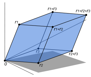
Volume and Jacobian determinant
As pointed out above, the absolute value of the determinant of real vectors is equal to the volume of the parallelepiped spanned by those vectors. As a consequence, if f: Rn → Rn is the linear map represented by the matrix A, and S is any measurable subset of Rn, then the volume of f(S) is given by |det(A)| times the volume of S. More generally, if the linear map f: Rn → Rm is represented by the m × n matrix A, then the n-dimensional volume of f(S) is given by:

By calculating the volume of the tetrahedron bounded by four points, they can be used to identify skew lines. The volume of any tetrahedron, given its vertices a, b, c, and d, is (1/6)·| det(a − b, b − c, c − d) |, or any other combination of pairs of vertices that would form a spanning tree over the vertices.
For a general differentiable function, much of the above carries over by considering the Jacobian matrix of f. For

the Jacobian is the n × n matrix whose entries are given by

Its determinant, the Jacobian determinant, appears in the higher-dimensional version of integration by substitution: for suitable functions f and an open subset U of Rn (the domain of f), the integral over f(U) of some other function φ: Rn → Rm is given by

The Jacobian also occurs in the inverse function theorem.
Vandermonde determinant (alternant)
The third order Vandermonde determinant is

In general, the nth-order Vandermonde determinant is[30]

where the right-hand side is the continued product of all the differences that can be formed from the n(n−1)/2 pairs of numbers taken from x1, x2, …, xn, with the order of the differences taken in the reversed order of the suffixes that are involved.
Circulants
Second order

Third order

where ω and ω2 are the complex cube roots of 1. In general, the nth-order circulant determinant is[30]

where ωj is an nth root of 1.
See also
- Dieudonné determinant
- Determinant identities
- Fuglede-Kadison determinant
- Functional determinant
- Immanant
- Matrix determinant lemma
- Permanent
- Pfaffian
- Slater determinant
Notes
- ↑ Serge Lang, Linear Algebra, 2nd Edition, Addison-Wesley, 1971, pp 173, 191.
- ↑ WildLinAlg episode 4, Norman J Wildberger, Univ. of New South Wales, 2010, lecture via youtube
- ↑ In a non-commutative setting left-linearity (compatibility with left-multiplication by scalars) should be distinguished from right-linearity. Assuming linearity in the columns is taken to be left-linearity, one would have, for non-commuting scalars a, b:
- ↑ § 0.8.2 of R. A. Horn & C. R. Johnson: Matrix Analysis 2nd ed. (2013) Cambridge University Press. ISBN 978-0-521-54823-6.
- ↑ Proofs can be found in http://www.ee.ic.ac.uk/hp/staff/dmb/matrix/proof003.html
- ↑ A proof can be found in the Appendix B of Kondratyuk, L. A.; Krivoruchenko, M. I. (1992). "Superconducting quark matter in SU(2) color group". Zeitschrift für Physik A. 344: 99–115. doi:10.1007/BF01291027.
- ↑ Habgood, Ken; Arel, Itamar (2012). "A condensation-based application of Cramerʼs rule for solving large-scale linear systems". Journal of Discrete Algorithms. 10: 98–109. doi:10.1016/j.jda.2011.06.007.
- ↑ These identities were taken from http://www.ee.ic.ac.uk/hp/staff/dmb/matrix/proof003.html
- ↑ Proofs are given in Silvester, J. R. (2000). "Determinants of Block Matrices" (PDF). Math. Gazette. 84: 460–467. JSTOR 3620776.
- ↑ Sothanaphan, Nat (January 2017). "Determinants of block matrices with noncommuting blocks". Linear Algebra and its Applications. 512: 202–218. doi:10.1016/j.laa.2016.10.004.
- ↑ § 0.8.10 of R. A. Horn & C. R. Johnson: Matrix Analysis 2nd ed. (2013) Cambridge University Press. ISBN 978-0-521-54823-6.
- ↑ Mac Lane, Saunders (1998), Categories for the Working Mathematician, Graduate Texts in Mathematics 5 ((2nd ed.) ed.), Springer-Verlag, ISBN 0-387-98403-8
- ↑ Varadarajan, V. S (2004), Supersymmetry for mathematicians: An introduction, ISBN 978-0-8218-3574-6.
- ↑ L. N. Trefethen and D. Bau, Numerical Linear Algebra (SIAM, 1997). e.g. in Lecture 1: "... we mention that the determinant, though a convenient notion theoretically, rarely finds a useful role in numerical algorithms."
- ↑ http://page.inf.fu-berlin.de/~rote/Papers/pdf/Division-free+algorithms.pdf
- ↑ Bunch, J. R.; Hopcroft, J. E. (1974). "Triangular Factorization and Inversion by Fast Matrix Multiplication". Mathematics of Computation. 28 (125): 231–236. doi:10.1090/S0025-5718-1974-0331751-8.
- ↑ Fang, Xin Gui; Havas, George (1997). "On the worst-case complexity of integer Gaussian elimination" (PDF). Proceedings of the 1997 international symposium on Symbolic and algebraic computation. ISSAC '97. Kihei, Maui, Hawaii, United States: ACM. pp. 28–31. doi:10.1145/258726.258740. ISBN 0-89791-875-4.
- ↑ Bareiss, Erwin (1968), "Sylvester's Identity and Multistep Integer-Preserving Gaussian Elimination" (PDF), Mathematics of computation, 22 (102): 565–578
- 1 2 3 Campbell, H: "Linear Algebra With Applications", pages 111–112. Appleton Century Crofts, 1971
- 1 2 Eves, H: "An Introduction to the History of Mathematics", pages 405, 493–494, Saunders College Publishing, 1990.
- ↑ A Brief History of Linear Algebra and Matrix Theory : http://darkwing.uoregon.edu/~vitulli/441.sp04/LinAlgHistory.html
- ↑ Cajori, F. A History of Mathematics p. 80
- ↑ Expansion of determinants in terms of minors: Laplace, Pierre-Simon (de) "Researches sur le calcul intégral et sur le systéme du monde," Histoire de l'Académie Royale des Sciences (Paris), seconde partie, pages 267–376 (1772).
- ↑ Muir, Sir Thomas, The Theory of Determinants in the historical Order of Development [London, England: Macmillan and Co., Ltd., 1906]. JFM 37.0181.02
- ↑ The first use of the word "determinant" in the modern sense appeared in: Cauchy, Augustin-Louis "Memoire sur les fonctions qui ne peuvent obtenir que deux valeurs égales et des signes contraires par suite des transpositions operées entre les variables qu'elles renferment," which was first read at the Institute de France in Paris on November 30, 1812, and which was subsequently published in the Journal de l'Ecole Polytechnique, Cahier 17, Tome 10, pages 29–112 (1815).
- ↑ Origins of mathematical terms: http://jeff560.tripod.com/d.html
- ↑ History of matrices and determinants: http://www-history.mcs.st-and.ac.uk/history/HistTopics/Matrices_and_determinants.html
- ↑ The first use of vertical lines to denote a determinant appeared in: Cayley, Arthur "On a theorem in the geometry of position," Cambridge Mathematical Journal, vol. 2, pages 267–271 (1841).
- ↑ History of matrix notation: http://jeff560.tripod.com/matrices.html
- 1 2 Gradshteyn, Izrail Solomonovich; Ryzhik, Iosif Moiseevich; Geronimus, Yuri Veniaminovich; Tseytlin, Michail Yulyevich (February 2007). "14.31". In Jeffrey, Alan; Zwillinger, Daniel. Table of Integrals, Series, and Products. Translated by Scripta Technica, Inc. (7 ed.). Academic Press, Inc. ISBN 0-12-373637-4. LCCN 2010481177. MR 2360010.

References
- Axler, Sheldon Jay (1997), Linear Algebra Done Right (2nd ed.), Springer-Verlag, ISBN 0-387-98259-0
- de Boor, Carl (1990), "An empty exercise" (PDF), ACM SIGNUM Newsletter, 25 (2): 3–7, doi:10.1145/122272.122273.
- Lay, David C. (August 22, 2005), Linear Algebra and Its Applications (3rd ed.), Addison Wesley, ISBN 978-0-321-28713-7
- Meyer, Carl D. (February 15, 2001), Matrix Analysis and Applied Linear Algebra, Society for Industrial and Applied Mathematics (SIAM), ISBN 978-0-89871-454-8
- Muir, Thomas (1960) [1933], A treatise on the theory of determinants, Revised and enlarged by William H. Metzler, New York, NY: Dover
- Poole, David (2006), Linear Algebra: A Modern Introduction (2nd ed.), Brooks/Cole, ISBN 0-534-99845-3
- G. Baley Price (1947) "Some identities in the theory of determinants", American Mathematical Monthly 54:75–90 MR 0019078
- Horn, R. A.; Johnson, C. R. (2013), Matrix Analysis (2nd ed.), Cambridge University Press, ISBN 978-0-521-54823-6
- Anton, Howard (2005), Elementary Linear Algebra (Applications Version) (9th ed.), Wiley International
- Leon, Steven J. (2006), Linear Algebra With Applications (7th ed.), Pearson Prentice Hall
External links
| The Wikibook Linear Algebra has a page on the topic of: Determinants |
- Suprunenko, D.A. (2001), "Determinant", in Hazewinkel, Michiel, Encyclopedia of Mathematics, Springer, ISBN 978-1-55608-010-4
- Weisstein, Eric W. "Determinant". MathWorld.
- O'Connor, John J.; Robertson, Edmund F., "Matrices and determinants", MacTutor History of Mathematics archive, University of St Andrews.
- Determinant Interactive Program and Tutorial
- Linear algebra: determinants. Compute determinants of matrices up to order 6 using Laplace expansion you choose.
- Matrices and Linear Algebra on the Earliest Uses Pages
- Determinants explained in an easy fashion in the 4th chapter as a part of a Linear Algebra course.
- Instructional Video on taking the determinant of an nxn matrix (Khan Academy)
- "The determinant". Essence of linear algebra – via YouTube.