Window function
In signal processing, a window function (also known as an apodization function or tapering function[1]) is a mathematical function that is zero-valued outside of some chosen interval. For instance, a function that is constant inside the interval and zero elsewhere is called a rectangular window, which describes the shape of its graphical representation. When another function or waveform/data-sequence is multiplied by a window function, the product is also zero-valued outside the interval: all that is left is the part where they overlap, the "view through the window".
In typical applications, the window functions used are non-negative, smooth, "bell-shaped" curves.[2] Rectangle, triangle, and other functions can also be used. A more general definition of window functions does not require them to be identically zero outside an interval, as long as the product of the window multiplied by its argument is square integrable, and, more specifically, that the function goes sufficiently rapidly toward zero.[3]
Applications
Applications of window functions include spectral analysis/modification/resynthesis,[4] the design of finite impulse response filters, as well as beamforming and antenna design.
Spectral analysis
The Fourier transform of the function cos ωt is zero, except at frequency ±ω. However, many other functions and waveforms do not have convenient closed-form transforms. Alternatively, one might be interested in their spectral content only during a certain time period.
In either case, the Fourier transform (or a similar transform) can be applied on one or more finite intervals of the waveform. In general, the transform is applied to the product of the waveform and a window function. Any window (including rectangular) affects the spectral estimate computed by this method.
Windowing
Windowing of a simple waveform like cos ωt causes its Fourier transform to develop non-zero values (commonly called spectral leakage) at frequencies other than ω. The leakage tends to be worst (highest) near ω and least at frequencies farthest from ω.
If the waveform under analysis comprises two sinusoids of different frequencies, leakage can interfere with the ability to distinguish them spectrally. If their frequencies are dissimilar and one component is weaker, then leakage from the stronger component can obscure the weaker one’s presence. But if the frequencies are similar, leakage can render them unresolvable even when the sinusoids are of equal strength. The rectangular window has excellent resolution characteristics for sinusoids of comparable strength, but it is a poor choice for sinusoids of disparate amplitudes. This characteristic is sometimes described as low dynamic range.
At the other extreme of dynamic range are the windows with the poorest resolution and sensitivity, which is the ability to reveal relatively weak sinusoids in the presence of additive random noise. That is because the noise produces a stronger response with high-dynamic-range windows than with high-resolution windows. Therefore, high-dynamic-range windows are most often justified in wideband applications, where the spectrum being analyzed is expected to contain many different components of various amplitudes.
In between the extremes are moderate windows, such as Hamming and Hann. They are commonly used in narrowband applications, such as the spectrum of a telephone channel. In summary, spectral analysis involves a trade-off between resolving comparable strength components with similar frequencies and resolving disparate strength components with dissimilar frequencies. That trade-off occurs when the window function is chosen.
Discrete-time signals
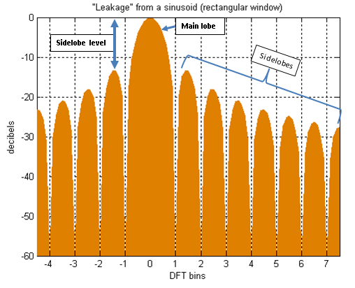
When the input waveform is time-sampled, instead of continuous, the analysis is usually done by applying a window function and then a discrete Fourier transform (DFT). But the DFT provides only a sparse sampling of the actual discrete-time Fourier transform (DTFT) spectrum. Figure 1 shows a portion of the DTFT for a rectangularly-windowed sinusoid. The actual frequency of the sinusoid is indicated as "0" on the horizontal axis. Everything else is leakage, exaggerated by the use of a logarithmic presentation. The unit of frequency is "DFT bins"; that is, the integer values on the frequency axis correspond to the frequencies sampled by the DFT. So the figure depicts a case where the actual frequency of the sinusoid coincides with a DFT sample, and the maximum value of the spectrum is accurately measured by that sample. When it misses the maximum value by some amount (up to ½ bin), the measurement error is referred to as scalloping loss (inspired by the shape of the peak). For a known frequency, such as a musical note or a sinusoidal test signal, matching the frequency to a DFT bin can be prearranged by choices of a sampling rate and a window length that results in an integer number of cycles within the window.
Noise bandwidth
The concepts of resolution and dynamic range tend to be somewhat subjective, depending on what the user is actually trying to do. But they also tend to be highly correlated with the total leakage, which is quantifiable. It is usually expressed as an equivalent bandwidth, B. It can be thought of as redistributing the DTFT into a rectangular shape with height equal to the spectral maximum and width B.[note 1][5] The more the leakage, the greater the bandwidth. It is sometimes called noise equivalent bandwidth or equivalent noise bandwidth, because it is proportional to the average power that will be registered by each DFT bin when the input signal contains a random noise component (or is just random noise). A graph of the power spectrum, averaged over time, typically reveals a flat noise floor, caused by this effect. The height of the noise floor is proportional to B. So two different window functions can produce different noise floors.
Processing gain and losses
In signal processing, operations are chosen to improve some aspect of quality of a signal by exploiting the differences between the signal and the corrupting influences. When the signal is a sinusoid corrupted by additive random noise, spectral analysis distributes the signal and noise components differently, often making it easier to detect the signal's presence or measure certain characteristics, such as amplitude and frequency. Effectively, the signal to noise ratio (SNR) is improved by distributing the noise uniformly, while concentrating most of the sinusoid's energy around one frequency. Processing gain is a term often used to describe an SNR improvement. The processing gain of spectral analysis depends on the window function, both its noise bandwidth (B) and its potential scalloping loss. These effects partially offset, because windows with the least scalloping naturally have the most leakage.
The figure at right depicts the effects of three different window functions on the same data set, comprising two equal strength sinusoids in additive noise. The frequencies of the sinusoids are chosen such that one encounters no scalloping and the other encounters maximum scalloping. Both sinusoids suffer less SNR loss under the Hann window than under the Blackman–Harris window. In general (as mentioned earlier), this is a deterrent to using high-dynamic-range windows in low-dynamic-range applications.
Filter design
Windows are sometimes used in the design of digital filters, in particular to convert an "ideal" impulse response of infinite duration, such as a sinc function, to a finite impulse response (FIR) filter design. That is called the window method.[6][7]
Rectangular window applications
Analysis of transients
When analyzing a transient signal in modal analysis, such as an impulse, a shock response, a sine burst, a chirp burst, or noise burst, where the energy vs time distribution is extremely uneven, the rectangular window may be most appropriate. For instance, when most of the energy is located at the beginning of the recording, a non-rectangular window attenuates most of the energy, degrading the signal-to-noise ratio.[8]
Harmonic analysis
One might wish to measure the harmonic content of a musical note from a particular instrument or the harmonic distortion of an amplifier at a given frequency. Referring again to Figure 1, we can observe that there is no leakage at a discrete set of harmonically-related frequencies sampled by the DFT. (The spectral nulls are actually zero-crossings, which cannot be shown on a logarithmic scale such as this.) This property is unique to the rectangular window, and it must be appropriately configured for the signal frequency, as described above.
Symmetry
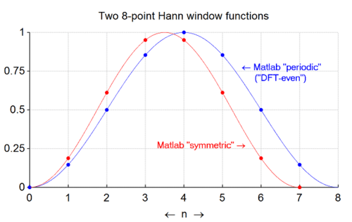
Window functions generated for digital filter design are symmetrical sequences, usually an odd length with a single maximum at the center. Windows for DFT/FFT usage, as in spectral analysis or time-frequency filtering, are often created by deleting the right-most coefficient of an odd-length, symmetrical window, making their discrete frequency spectrum purely real.[9] These are known as periodic[10] or DFT-even.[11] Such a window is generated by the MATLAB function hann(512,'periodic') for instance. To generate it with the formula in this article (below), the window length (N) is 513, and the 513th coefficient of the generated sequence is discarded.
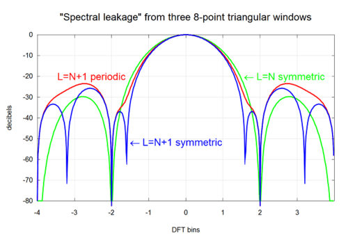
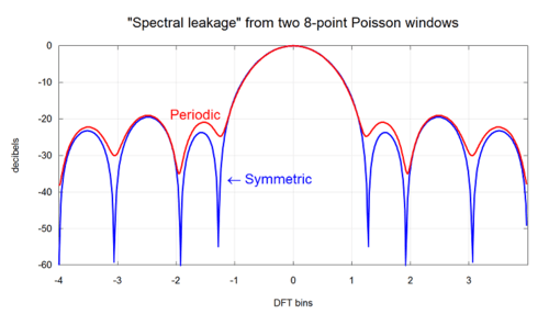
For a window function with zero-valued end-points, deleting one or both end-points has no effect on its DTFT. But the function designed for N+1 samples, instead of N, typically has a slightly narrower main lobe, slightly higher sidelobes, and a slightly lower noise bandwidth. Similarly, deleting both zeros from a function designed for N+2 samples further amplifies those effects. For a window function with non-zero end-points, such as triangular or Poisson, deleting one of them can result in higher sidelobes and noise bandwidth with little or no main lobe improvement.
There is also a cosmetic result of truncating an N+1 sample symmetric window. It happens when we sample the DTFT only at intervals of cycles/sample, which is the effect of an N-point DFT. The baseline width of the N+1 sample window with zero-valued end-points is just N sample-intervals. That usually means the DTFT zero-crossings, which create the fine-grained sidelobe structure away from the main lobe, occur at an interval that asymptotically approaches the same interval as the DFT samples. When that allows most of the DFT samples to occur at or near the zero-crossings, it creates an illusion of little or no spectral leakage. But such a plot only reveals the leakage into the DFT bins from a sinusoid whose frequency is also an integer DFT bin. The unseen sidelobes reveal the leakage to expect from sinusoids at other frequencies.[12] That is why it's important to present the continuous function (as seen below) and choose a window that suppresses the sidelobes to an acceptable level.

A list of window functions
Terminology:
- N represents the width, in samples, of a discrete-time, symmetrical window function When N is an odd number, the non-flat windows have a singular maximum point. When N is even, they have a double maximum.
- It is sometimes useful to express as a sequence of samples of the lagged version of a zero-phase function:
![w[n],\ 0\leq n\leq N-1.](../I/m/09da5cec88620b552fcb62dc2e96dc0359674e73.svg)
![w[n]](../I/m/2a4e3e5afc2a8c6da9020b8c6b21450959101a18.svg)
![w[n]=\ w_{0}\left(n-{\frac {N-1}{2}}\right),\ 0\leq n\leq N-1.](../I/m/0813f9b0d390192091a4ce100a9d9ce7949922bc.svg)
- Each figure label includes the corresponding noise equivalent bandwidth metric (B),[note 1] in units of DFT bins.
B-spline windows
B-spline windows can be obtained as k-fold convolutions of the rectangular window. They include the rectangular window itself (k = 1), the triangular window (k = 2) and the Parzen window (k = 4).[14] Alternative definitions sample the appropriate normalized B-spline basis functions instead of convolving discrete-time windows. A kth order B-spline basis function is a piece-wise polynomial function of degree k−1 that is obtained by k-fold self-convolution of the rectangular function.
Rectangular window
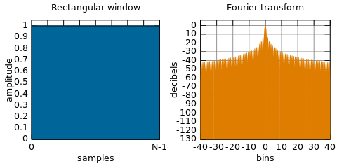
The rectangular window (sometimes known as the boxcar or Dirichlet window) is the simplest window, equivalent to replacing all but N values of a data sequence by zeros, making it appear as though the waveform suddenly turns on and off:

Other windows are designed to moderate these sudden changes, which reduces scalloping loss and improves dynamic range, as described above (Window function#Spectral analysis).
The rectangular window is the 1st order B-spline window as well as the 0th power cosine window.
Triangular window
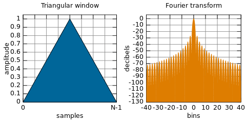
Triangular windows are given by:

where L can be N,[11][16] N+1,[17] or N-1.[18] The last one is also known as Bartlett window or Fejér window. All three definitions converge at large N.
The triangular window is the 2nd order B-spline window and can be seen as the convolution of two N/2 width rectangular windows. The Fourier transform of the result is the squared values of the transform of the half-width rectangular window.
Parzen window
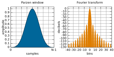
The Parzen window, also known as the de la Vallée Poussin window,[11] is the 4th order B-spline window given by:

Other polynomial windows
Welch window
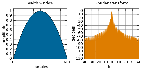
The Welch window consists of a single parabolic section:
- .[17]

The defining quadratic polynomial reaches a value of zero at the samples just outside the span of the window.
Generalized Hamming windows
Generalized Hamming windows are of the form:
- .

The periodic/DFT-even forms have only three non-zero DFT coefficients and share the benefits of a sparse frequency domain representation with higher-order generalized cosine windows.
Hann (Hanning) window
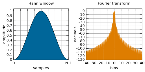
The Hann window named after Julius von Hann and also known as the Hanning (for being similar in name and form to the Hamming window), von Hann and the raised cosine window is defined by (with hav for the haversine function):[19]

The ends of the cosine just touch zero, so the side-lobes roll off at about 18 dB per octave.[20]
Hamming window
.svg.png)
The window with these particular coefficients was proposed by Richard W. Hamming. The window is optimized to minimize the maximum (nearest) side lobe, giving it a height of about one-fifth that of the Hann window.[21][22]

with

instead of both constants being equal to 1/2 in the Hann window. The constants are approximations of values α = 25/46 and β = 21/46, which cancel the first sidelobe of the Hann window by placing a zero at frequency 5π/(N − 1).[11] Approximation of the constants to two decimal places substantially lowers the level of sidelobes,[11] to a nearly equiripple condition.[22] In the equiripple sense, the optimal values for the coefficients are α = 0.53836 and β = 0.46164.[22][23]
- zero-phase version:

Higher-order generalized cosine windows
Windows of the form:

have only 2K + 1 non-zero DFT coefficients, which makes them good choices for applications that require windowing by convolution in the frequency-domain. In those applications, the DFT of the unwindowed data vector is needed for a different purpose than spectral analysis. (see Overlap-save method). Generalized cosine windows with just two terms (K = 1) belong in the subfamily generalized Hamming windows.
Blackman windows
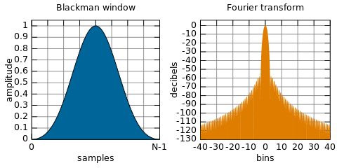
Blackman windows are defined as:


By common convention, the unqualified term Blackman window refers to Blackman's "not very serious proposal" of α = 0.16 (a0 = 0.42, a1 = 0.5, a2 = 0.08), which closely approximates the "exact Blackman",[24] with a0 = 7938/18608 ≈ 0.42659, a1 = 9240/18608 ≈ 0.49656, and a2 = 1430/18608 ≈ 0.076849.[25] These exact values place zeros at the third and fourth sidelobes,[11] but result in a discontinuity at the edges and a 6 dB/oct fall-off. The truncated coefficients do not null the sidelobes as well, but have an improved 18 dB/oct fall-off.[11][26]
Nuttall window, continuous first derivative
.svg.png)
Considering n as a real number, the Nuttall window function and its first derivative are continuous everywhere. That is, the function goes to 0 at n = 0, unlike the Blackman–Nuttall and Blackman–Harris windows, which have a small positive value at zero (at "step" from the zero outside the window), like the Hamming window. The Blackman window defined via α is also continuous with continuous derivative at the edge, but the described "exact Blackman window" is not.


Blackman–Nuttall window
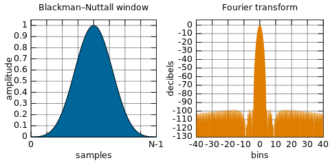

Blackman–Harris window
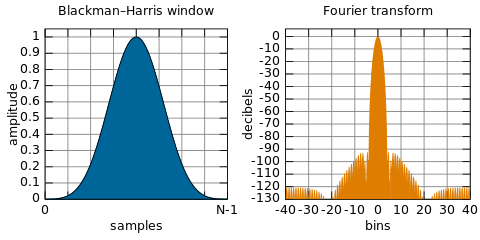
A generalization of the Hamming family, produced by adding more shifted sinc functions, meant to minimize side-lobe levels[27][28]

Flat top window
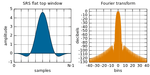
A flat top window is a partially negative-valued window that has minimal scalloping loss in the frequency domain. Such windows have been made available in spectrum analyzers for the measurement of amplitudes of sinusoidal frequency components.[15][29] Drawbacks of the broad bandwidth are poor frequency resolution and high noise bandwidth.
Flat top windows can be designed using low-pass filter design methods,[29] or they may be of the usual sum-of-cosine-terms variety.[15] An example of the latter is the flat top window available in the Stanford Research Systems (SRS) SR785 spectrum analyzer:


Rife–Vincent window
Rife and Vincent define three classes of windows constructed as sums of cosines; the classes are generalizations of the Hanning window.[30] Their order-P windows are of the form (normalized to have unity average as opposed to unity max as the windows above are):
- .

For order 1, this formula can match the Hanning window for a1 = −1; this is the Rife–Vincent class-I window, defined by minimizing the high-order sidelobe amplitude. The class-I order-2 Rife–Vincent window has a1 = −4/3 and a2 = 1/3. Coefficients for orders up to 4 are tabulated.[31] For orders greater than 1, the Rife–Vincent window coefficients can be optimized for class II, meaning minimized main-lobe width for a given maximum side-lobe, or for class III, a compromise for which order 2 resembles Blackmann's window.[31][32] Given the wide variety of Rife–Vincent windows, plots are not given here.
Power-of-cosine windows
Window functions in the power-of-cosine family are of the form:

The rectangular window (α = 0), the cosine window (α = 1), and the Hann window (α = 2) are members of this family.
Cosine window


The cosine window is also known as the sine window. Cosine window describes the shape of

A cosine window convolved by itself is known as the Bohman window.
Adjustable windows
Gaussian window
.svg.png)
The Fourier transform of a Gaussian is also a Gaussian (it is an eigenfunction of the Fourier Transform). Since the Gaussian function extends to infinity, it must either be truncated at the ends of the window, or itself windowed with another zero-ended window.[33]
Since the log of a Gaussian produces a parabola, this can be used for nearly exact quadratic interpolation in frequency estimation.[33][34][35]


The standard deviation of the Gaussian function is σ(N−1)/2 sampling periods.
.svg.png)
Confined Gaussian window
The confined Gaussian window yields the smallest possible root mean square frequency width σω for a given temporal width σt.[36] These windows optimize the RMS time-frequency bandwidth products. They are computed as the minimum eigenvectors of a parameter-dependent matrix. The confined Gaussian window family contains the cosine window and the Gaussian window in the limiting cases of large and small σt, respectively.
.svg.png)
Approximate confined Gaussian window
A confined Gaussian window of temporal width σt is well approximated by:[36]
![w(n)=G(n)-{\frac {G(-{\tfrac {1}{2}})[G(n+N)+G(n-N)]}{G(-{\tfrac {1}{2}}+N)+G(-{\tfrac {1}{2}}-N)}}](../I/m/6c40355672e7157d120b21eb0bb483e2a764f957.svg)
with the Gaussian:

The temporal width of the approximate window is asymptotically equal to σt for σt < 0.14 N.[36]
Generalized normal window
A more generalized version of the Gaussian window is the generalized normal window.[37] Retaining the notation from the Gaussian window above, we can represent this window as

for any even . At , this is a Gaussian window and as approaches , this approximates to a rectangular window. The Fourier transform of this window does not exist in a closed form for a general . However, it demonstrates the other benefits of being smooth, adjustable bandwidth. Like the Tukey window discussed later, this window naturally offers a "flat top" to control the amplitude attenuation of a time-series (on which we don't have a control with Gaussian window). In essence, it offers a good (controllable) compromise, in terms of spectral leakage, frequency resolution and amplitude attenuation, between the Gaussian window and the rectangular window. See also [38] for a study on time-frequency representation of this window (or function).


Tukey window
.svg.png)
The Tukey window,[11][39] also known as the tapered cosine window, can be regarded as a cosine lobe of width αN/2 that is convolved with a rectangular window of width (1 − α/2)N.
![{\displaystyle w(n)=\left\{{\begin{matrix}{\frac {1}{2}}\left[1+\cos \left(\pi \left({\frac {2n}{\alpha (N-1)}}-1\right)\right)\right]&0\leqslant n<{\frac {\alpha (N-1)}{2}}\\1&{\frac {\alpha (N-1)}{2}}\leqslant n\leqslant (N-1)(1-{\frac {\alpha }{2}})\\{\frac {1}{2}}\left[1+\cos \left(\pi \left({\frac {2n}{\alpha (N-1)}}-{\frac {2}{\alpha }}+1\right)\right)\right]&(N-1)(1-{\frac {\alpha }{2}})<n\leqslant (N-1)\\\end{matrix}}\right.}](../I/m/82550244afcf7641f0c913cebb7355eedfac2ca7.svg)
or expressed with the havercosine (hvc) function:

At α = 0 it becomes rectangular, and at α = 1 it becomes a Hann window.
Planck-taper window
.svg.png)
The so-called "Planck-taper" window is a bump function that has been widely used[40] in the theory of partitions of unity in manifolds. It is smooth (a function) everywhere, but is exactly zero outside of a compact region, exactly one over an interval within that region, and varies smoothly and monotonically between those limits. Its use as a window function in signal processing was first suggested in the context of gravitational-wave astronomy, inspired by the Planck distribution.[41] It is defined as a piecewise function:


where
![{\displaystyle Z_{\pm }(n;\epsilon )=2\epsilon \left[{\frac {1}{1\pm (2n/(N-1)-1)}}+{\frac {1}{1-2\epsilon \pm (2n/(N-1)-1)}}\right].}](../I/m/8dacd2db57d0b295cf4589148e5f8fb70bba7fba.svg)
The amount of tapering (the region over which the function is exactly 1) is controlled by the parameter ε, with smaller values giving sharper transitions.
DPSS or Slepian window
.svg.png)
.svg.png)
The DPSS (discrete prolate spheroidal sequence) or Slepian window is used to maximize the energy concentration in the main lobe.[42]
The main lobe ends at a bin given by the parameter α.[43]
Kaiser window
.svg.png)
.svg.png)
The Kaiser, or Kaiser-Bessel, window is a simple approximation of the DPSS window using Bessel functions, discovered by Jim Kaiser.[44][45][43][46]

where I0 is the zero-th order modified Bessel function of the first kind. Variable parameter α determines the tradeoff between main lobe width and side lobe levels of the spectral leakage pattern. The main lobe width, in between the nulls, is given by in units of DFT bins,[47] and a typical value of α is 3.

- Sometimes the formula for w(n) is written in terms of a parameter [46]
- zero-phase version:


Dolph–Chebyshev window
.svg.png)
Minimizes the Chebyshev norm of the side-lobes for a given main lobe width.[48]
The zero-phase Dolph–Chebyshev window function w0(n) is usually defined in terms of its real-valued discrete Fourier transform, W0(k):
![{\begin{aligned}W_{0}(k)&={\frac {\cos\{N\cos ^{-1}[\beta \cos({\frac {\pi k}{N}})]\}}{\cosh[N\cosh ^{-1}(\beta )]}}\\\beta &=\cosh[{\frac {1}{N}}\cosh ^{-1}(10^{\alpha })],\end{aligned}}](../I/m/35a73585f37d9a66f1edcec09a31e53a17dc3762.svg)
where the parameter α sets the Chebyshev norm of the sidelobes to −20α decibels.[48]
The window function can be calculated from W0(k) by an inverse discrete Fourier transform (DFT):[48]

The lagged version of the window, with 0 ≤ n ≤ N−1, can be obtained by:

which for even values of N must be computed as follows:
![{\begin{aligned}w_{0}\left(n-{\frac {N-1}{2}}\right)={\frac {1}{N}}\sum _{k=0}^{N-1}W_{0}(k)\cdot e^{i2\pi k(n-{\frac {N-1}{2}})/N}={\frac {1}{N}}\sum _{k=0}^{N-1}\left[(-e^{\frac {i\pi }{N}})^{k}\cdot W_{0}(k)\right]e^{i2\pi kn/N},\end{aligned}}](../I/m/b4b8f79e4d8059cce8348694acd522af5fb9afc8.svg)
which is an inverse DFT of

Variations:
- Due to the equiripple condition, the time-domain window has discontinuities at the edges. An approximation that avoids them, by allowing the equiripples to drop off at the edges, is a Taylor window.
- An alternative to the inverse DFT definition is also available..
Ultraspherical window
.svg.png)
The Ultraspherical window was introduced in 1984 by Roy Streit[49] and has application in antenna array design,[50] non-recursive filter design,[49] and spectrum analysis.[51]
Like other adjustable windows, the Ultraspherical window has parameters that can be used to control its Fourier transform main-lobe width and relative side-lobe amplitude. Uncommon to other windows, it has an additional parameter which can be used to set the rate at which side-lobes decrease (or increase) in amplitude.[51][52]
The window can be expressed in the time-domain as follows:[51]
![{\begin{aligned}w\left(n\right)={\frac {1}{N}}\left[C_{N-1}^{\mu }(x_{0})+\sum _{k=1}^{\frac {N-1}{2}}C_{N-1}^{\mu }\left(x_{0}\cos {\frac {k\pi }{N}}\right)\cos {\frac {2n\pi k}{N}}\right]\end{aligned}}](../I/m/aa645bf40c32be36ab539797ffe5062b527fdc1b.svg)
where is the Ultraspherical polynomial of degree N, and and control the side-lobe patterns.[51]


Certain specific values of yield other well-known windows: and give the Dolph–Chebyshev and Saramäki windows respectively.[49] See here for illustration of Ultraspherical windows with varied parametrization.


Exponential or Poisson window
.svg.png)
.svg.png)
The Poisson window, or more generically the exponential window increases exponentially towards the center of the window and decreases exponentially in the second half. Since the exponential function never reaches zero, the values of the window at its limits are non-zero (it can be seen as the multiplication of an exponential function by a rectangular window [53]). It is defined by

where τ is the time constant of the function. The exponential function decays as e ≃ 2.71828 or approximately 8.69 dB per time constant.[54] This means that for a targeted decay of D dB over half of the window length, the time constant τ is given by

Hybrid windows
Window functions have also been constructed as multiplicative or additive combinations of other windows.
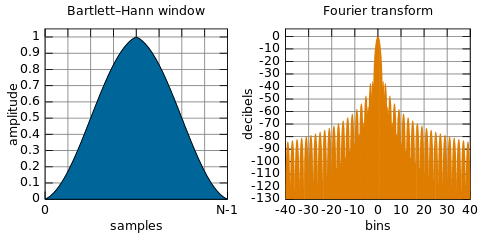
Bartlett–Hann window


Planck–Bessel window
.svg.png)
A Planck-taper window multiplied by a Kaiser window which is defined in terms of a modified Bessel function. This hybrid window function was introduced to decrease the peak side-lobe level of the Planck-taper window while still exploiting its good asymptotic decay.[55] It has two tunable parameters, ε from the Planck-taper and α from the Kaiser window, so it can be adjusted to fit the requirements of a given signal.
Hann–Poisson window
.svg.png)
A Hann window multiplied by a Poisson window, which has no side-lobes, in the sense that its Fourier transform drops off forever away from the main lobe. It can thus be used in hill climbing algorithms like Newton's method.[56] The Hann–Poisson window is defined by:

where α is a parameter that controls the slope of the exponential.
Other windows
Lanczos window
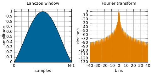

- used in Lanczos resampling
- for the Lanczos window, is defined as
- also known as a sinc window, because:


- is the main lobe of a normalized sinc function

Comparison of windows
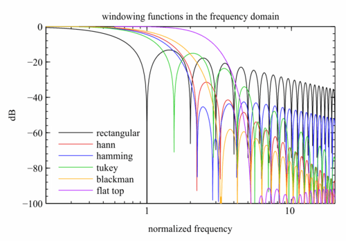
When selecting an appropriate window function for an application, this comparison graph may be useful. The frequency axis has units of FFT "bins" when the window of length N is applied to data and a transform of length N is computed. For instance, the value at frequency ½ "bin" (third tick mark) is the response that would be measured in bins k and k+1 to a sinusoidal signal at frequency k+½. It is relative to the maximum possible response, which occurs when the signal frequency is an integer number of bins. The value at frequency ½ is referred to as the maximum scalloping loss of the window, which is one metric used to compare windows. The rectangular window is noticeably worse than the others in terms of that metric.
Other metrics that can be seen are the width of the main lobe and the peak level of the sidelobes, which respectively determine the ability to resolve comparable strength signals and disparate strength signals. The rectangular window (for instance) is the best choice for the former and the worst choice for the latter. What cannot be seen from the graphs is that the rectangular window has the best noise bandwidth, which makes it a good candidate for detecting low-level sinusoids in an otherwise white noise environment. Interpolation techniques, such as zero-padding and frequency-shifting, are available to mitigate its potential scalloping loss.
Overlapping windows
When the length of a data set to be transformed is larger than necessary to provide the desired frequency resolution, a common practice is to subdivide it into smaller sets and window them individually. To mitigate the "loss" at the edges of the window, the individual sets may overlap in time. See Welch method of power spectral analysis and the modified discrete cosine transform.
Two-dimensional windows
Two-dimensional windows are used in, e.g., image processing. They can be constructed from one-dimensional windows in either of two forms.[57]
The separable form, is trivial to compute. The radial form, , which involves the radius , is isotropic, independent on the orientation of the coordinate axes. Only the Gaussian function is both separable and isotropic.[58] The separable forms of all other window functions have corners that depend on the choice of the coordinate axes. The isotropy/anisotropy of a two-dimensional window function is shared by its two-dimensional Fourier transform. The difference between the separable and radial forms is akin to the result of diffraction from rectangular vs. circular appertures, which can be visualized in terms of the product of two sinc functions vs. an Airy function, respectively.


See also
| Wikimedia Commons has media related to Window function. |
- Spectral leakage
- Multitaper
- Apodization
- Welch method
- Short-time Fourier transform
- Window design method
- Kolmogorov–Zurbenko filter
Notes
- 1 2 Mathematically, the noise equivalent bandwidth of transfer function H is the bandwidth of an ideal rectangular filter with the same peak gain as H that would pass the same power with white noise input. In the units of frequency f (e.g. hertz), it is given by:

References
- ↑ Weisstein, Eric W. (2003). CRC Concise Encyclopedia of Mathematics. CRC Press. ISBN 1-58488-347-2.
- ↑ Roads, Curtis (2002). Microsound. MIT Press. ISBN 0-262-18215-7.
- ↑ Cattani, Carlo; Rushchitsky, Jeremiah (2007). Wavelet and Wave Analysis As Applied to Materials With Micro Or Nanostructure. World Scientific. ISBN 981-270-784-0.
- ↑ "Overlap-Add (OLA) STFT Processing | Spectral Audio Signal Processing". www.dsprelated.com. Retrieved 2016-08-07.
The window is applied twice: once before the FFT (the "analysis window") and secondly after the inverse FFT prior to reconstruction by overlap-add (the so-called "synthesis window"). ... More generally, any positive COLA window can be split into an analysis and synthesis window pair by taking its square root.
- ↑ Carlson, A. Bruce (1986). Communication Systems: An Introduction to Signals and Noise in Electrical Communication. McGraw-Hill. ISBN 0-07-009960-X.
- ↑ "FIR Filters by Windowing - The Lab Book Pages". www.labbookpages.co.uk. Retrieved 2016-04-13.
- ↑ Mastering Windows: Improving Reconstruction
- ↑ The Fundamentals of Signal Analysis Application Note 243
- ↑ Harris, F. J. (1978-01-01). "On the use of windows for harmonic analysis with the discrete Fourier transform". Proceedings of the IEEE. 66 (1): 51–83. doi:10.1109/PROC.1978.10837. ISSN 0018-9219.
The DFT of the same sequence is a set of samples of the finite Fourier transform, yet these samples exhibit an imaginary component equal to zero.
- ↑ "Hann (Hanning) window - MATLAB hann". www.mathworks.com. Retrieved 2016-04-13.
- 1 2 3 4 5 6 7 8 9 10 11 12 13 14 15 Harris, Fredric J. (Jan 1978). "On the use of Windows for Harmonic Analysis with the Discrete Fourier Transform" (PDF). Proceedings of the IEEE. 66 (1): 51–83. doi:10.1109/PROC.1978.10837. The fundamental 1978 paper on FFT windows by Harris, which specified many windows and introduced key metrics used to compare them.
- ↑ Harris, Fredric J. (Jan 1978), fig 10, p 178.
- ↑ Rorabaugh, C. Britton (October 1998). DSP Primer. Primer series. McGraw-Hill Professional. p. 196. ISBN 0070540047.
- ↑ Toraichi, K.; Kamada, M.; Itahashi, S.; Mori, R. (1989). "Window functions represented by B-spline functions". IEEE Transactions on Acoustics, Speech, and Signal Processing. 37: 145. doi:10.1109/29.17517.
- 1 2 3 4 5 6 7 8 9 10 11 12 Heinzel, G.; Rüdiger, A.; Schilling, R. (2002). Spectrum and spectral density estimation by the Discrete Fourier transform (DFT), including a comprehensive list of window functions and some new flat-top windows (Technical report). Max Planck Institute (MPI) für Gravitationsphysik / Laser Interferometry & Gravitational Wave Astronomy. 395068.0. Retrieved 2013-02-10.
- ↑ "Triangular window - MATLAB triang". www.mathworks.com. Retrieved 2016-04-13.
- 1 2 Welch, P. (1967). "The use of fast Fourier transform for the estimation of power spectra: A method based on time averaging over short, modified periodograms". IEEE Transactions on Audio and Electroacoustics. 15 (2): 70. doi:10.1109/TAU.1967.1161901.
- ↑ "Bartlett Window". ccrma.stanford.edu. Retrieved 2016-04-13.
- ↑ "Hann (Hanning) window - MATLAB hann". www.mathworks.com. Retrieved 2016-04-13.
- ↑ "Hann or Hanning or Raised Cosine". ccrma.stanford.edu. Retrieved 2016-04-13.
- ↑ Enochson, Loren D.; Otnes, Robert K. (1968). Programming and Analysis for Digital Time Series Data. U.S. Dept. of Defense, Shock and Vibration Info. Center. p. 142.
- 1 2 3 "Hamming Window". ccrma.stanford.edu. Retrieved 2016-04-13.
- ↑ Nuttall, A. H. (February 1981). "Some windows with very good sidelobe behavior". IEEE Transactions on Acoustics, Speech, Signal Processing. ASSP-29: 84–91.
- ↑ W., Weisstein, Eric. "Blackman Function". mathworld.wolfram.com. Retrieved 2016-04-13.
- ↑ "Characteristics of Different Smoothing Windows - NI LabVIEW 8.6 Help". zone.ni.com. Retrieved 2016-04-13.
- ↑ Blackman, R. B.; Tukey, J. W. (1959-01-01). The Measurement of Power Spectra from the Point of View of Communications Engineering. Dover Publications. p. 99. ISBN 9780486605074.
- ↑ "Blackman-Harris Window Family". ccrma.stanford.edu. Retrieved 2016-04-13.
- ↑ "Three-Term Blackman-Harris Window". ccrma.stanford.edu. Retrieved 2016-04-13.
- 1 2 Smith, Steven W. (2011). The Scientist and Engineer's Guide to Digital Signal Processing. San Diego, California, USA: California Technical Publishing. Retrieved 2013-02-14.
- ↑ Rife, David C.; Vincent, G. A. (1970), "Use of the discrete Fourier transform in the measurement of frequencies and levels of tones", Bell Syst. Tech. J., 49 (2): 197–228, doi:10.1002/j.1538-7305.1970.tb01766.x
- 1 2 Andria, Gregorio; Savino, Mario; Trotta, Amerigo (1989), "Windows and interpolation algorithms to improve electrical measurement accuracy", Instrumentation and Measurement, IEEE Transactions on, 38 (4): 856–863, doi:10.1109/19.31004
- ↑ Schoukens, Joannes; Pintelon, Rik; Van Hamme, Hugo (1992), "The interpolated fast Fourier transform: a comparative study", Instrumentation and Measurement, IEEE Transactions on, 41 (2): 226–232, doi:10.1109/19.137352
- 1 2 "Gaussian Window and Transform". ccrma.stanford.edu. Retrieved 2016-04-13.
- ↑ "Matlab for the Gaussian Window". ccrma.stanford.edu. Retrieved 2016-04-13.
Note that, on a dB scale, Gaussians are quadratic. This means that parabolic interpolation of a sampled Gaussian transform is exact. ... quadratic interpolation of spectral peaks may be more accurate on a log-magnitude scale (e.g., dB) than on a linear magnitude scale
- ↑ "Quadratic Interpolation of Spectral Peaks". ccrma.stanford.edu. Retrieved 2016-04-13.
- 1 2 3 Starosielec, S.; Hägele, D. (2014). "Discrete-time windows with minimal RMS bandwidth for given RMS temporal width". Signal Processing. Elsevier. doi:10.1016/j.sigpro.2014.03.033.
- ↑ Debejyo Chakraborty and Narayan Kovvali Generalized Normal Window for Digital Signal Processing in IEEE International Conference on Acoustics, Speech and Signal Processing (ICASSP) 2013 6083 -- 6087 doi:10.1109/ICASSP.2013.6638833
- ↑ Diethorn, E.J., "The generalized exponential time-frequency distribution," Signal Processing, IEEE Transactions on , vol.42, no.5, pp.1028,1037, May 1994 doi: 10.1109/78.295214
- ↑ Tukey, J.W. (1967). "An introduction to the calculations of numerical spectrum analysis". Spectral Analysis of Time Series: 25–46.
- ↑ Tu, Loring W. (2008). "Bump Functions and Partitions of Unity". An Introduction to Manifolds. New York: Springer. pp. 127–134. ISBN 978-0-387-48098-5. Retrieved 2013-10-04.
- ↑ McKechan, D. J. A.; Robinson, C.; Sathyaprakash, B. S. (21 April 2010). "A tapering window for time-domain templates and simulated signals in the detection of gravitational waves from coalescing compact binaries". Classical and Quantum Gravity. 27 (8): 084020. arXiv:1003.2939
 . Bibcode:2010CQGra..27h4020M. doi:10.1088/0264-9381/27/8/084020.
 - ↑ "Slepian or DPSS Window". ccrma.stanford.edu. Retrieved 2016-04-13.
- 1 2 "Kaiser and DPSS Windows Compared". ccrma.stanford.edu. Retrieved 2016-04-13.
- ↑ Kaiser, James F.; Kuo, Franklin F. (1966). System Analysis by Digital Computer. John Wiley and Sons. pp. 232–235.
This family of window functions was "discovered" by Kaiser in 1962 following a discussion with B. F. Logan of the Bell Telephone Laboratories. ... Another valuable property of this family ... is that they also approximate closely the prolate spheroidal wave functions of order zero
- ↑ Kaiser, James F. (November 1964). "A family of window functions having nearly ideal properties". unpublished memorandum. Murray Hill, NJ: Bell Telephone Laboratories.
- 1 2 "Kaiser Window". ccrma.stanford.edu. Retrieved 2016-04-13.
- ↑ Kaiser, James F.; Schafer, Ronald W. (1980). "On the use of the I0-sinh window for spectrum analysis". IEEE Transactions on Acoustics, Speech, and Signal Processing. 28: 105–107. doi:10.1109/TASSP.1980.1163349.
- 1 2 3 "Dolph-Chebyshev Window". ccrma.stanford.edu. Retrieved 2016-04-13.
- 1 2 3 Kabal, Peter (2009). "Time Windows for Linear Prediction of Speech" (PDF). Technical Report, Dept. Elec. & Comp. Eng., McGill University (2a): 31. Retrieved 2 February 2014.
- ↑ Streit, Roy (1984). "A two-parameter family of weights for nonrecursive digital filters and antennas". Transactions of ASSP. 32: 108–118. doi:10.1109/tassp.1984.1164275.
- 1 2 3 4 Deczky, Andrew (2001). "Unispherical Windows". IEEE Int. Symp. on Circuits and Systems. II: 85–88. doi:10.1109/iscas.2001.921012.
- ↑ Bergen, S. W. A.; Antoniou, A. (2004). "Design of Ultraspherical Window Functions with Prescribed Spectral Characteristics". EURASIP Journal on Applied Signal Processing. 2004 (13): 2053–2065. doi:10.1155/S1110865704403114.
- ↑ Smith, Julius O. III (April 23, 2011), Spectral Audio Signal Processing, retrieved November 22, 2011
- ↑ Gade, Svend; Herlufsen, Henrik (1987). "Technical Review No 3-1987: Windows to FFT analysis (Part I)" (PDF). Brüel & Kjær. Retrieved November 22, 2011.
- ↑ Berry, C. P. L.; Gair, J. R. (12 December 2012). "Observing the Galaxy's massive black hole with gravitational wave bursts". Monthly Notices of the Royal Astronomical Society. 429 (1): 589–612. arXiv:1210.2778. Bibcode:2013MNRAS.429..589B. doi:10.1093/mnras/sts360.
- ↑ "Hann-Poisson Window". ccrma.stanford.edu. Retrieved 2016-04-13.
- ↑ Matt A. Bernstein, Kevin Franklin King, Xiaohong Joe Zhou (2007), Handbook of MRI Pulse Sequences, Elsevier; p.495-499.
- ↑ Awad, A. I.; Baba, K. (2011). "An Application for Singular Point Location in Fingerprint Classification". Digital Information Processing and Communications. Communications in Computer and Information Science. 188. p. 262. doi:10.1007/978-3-642-22389-1_24. ISBN 978-3-642-22388-4.
Further reading
- Albrecht, Hans-Helge (2012). Tailored minimum sidelobe and minimum sidelobe cosine-sum windows. A catalog. doi:10.7795/110.20121022aa.
- Bergen, S. W. A.; Antoniou, A. (2004). "Design of Ultraspherical Window Functions with Prescribed Spectral Characteristics". EURASIP Journal on Applied Signal Processing. 2004 (13): 2053–2065. doi:10.1155/S1110865704403114.
- Bergen, S. W. A.; Antoniou, A. (2005). "Design of Nonrecursive Digital Filters Using the Ultraspherical Window Function". EURASIP Journal on Applied Signal Processing. 2005 (12): 1910–1922. doi:10.1155/ASP.2005.1910.
- Nuttall, Albert H. (February 1981). "Some Windows with Very Good Sidelobe Behavior". IEEE Transactions on Acoustics, Speech, and Signal Processing. 29 (1): 84–91. doi:10.1109/TASSP.1981.1163506. Extends Harris' paper, covering all the window functions known at the time, along with key metric comparisons.
- Oppenheim, Alan V.; Schafer, Ronald W.; Buck, John A. (1999). Discrete-time signal processing. Upper Saddle River, N.J.: Prentice Hall. pp. 468–471. ISBN 0-13-754920-2.
- US patent 7065150, Park, Young-Seo, "System and method for generating a root raised cosine orthogonal frequency division multiplexing (RRC OFDM) modulation", published 2003, issued 2006
External links
- LabView Help, Characteristics of Smoothing Filters, http://zone.ni.com/reference/en-XX/help/371361B-01/lvanlsconcepts/char_smoothing_windows/
- Evaluation of Various Window Function using Multi-Instrument, http://www.multi-instrument.com/doc/D1003/Evaluation_of_Various_Window_Functions_using_Multi-Instrument_D1003.pdf