Born coordinates

Space-time geometry of Born coordinates. Red lines are world lines (congruence) of points on disc. Interlacing blue and grey stripes show change of T. Orange curves ( / \ ) are time-like curves with fixed R.

In relativistic physics, the Born coordinate chart is a coordinate chart for (part of) Minkowski spacetime, the flat spacetime of special relativity. It is often used to analyze the physical experience of observers who ride on a ring or disk rigidly rotating at relativistic speeds. This chart is often attributed to Max Born, due to his 1909 work on the relativistic physics of a rotating body – see Born rigidity.

Langevin observers in the cylindrical chart

To motivate the Born chart, we first consider the family of Langevin observers represented in an ordinary cylindrical coordinate chart for Minkowski spacetime. The world lines of these observers form a timelike congruence which is rigid in the sense of having a vanishing expansion tensor. They represent observers who rotate rigidly around an axis of cylindrical symmetry.

From the line element

ds^{2}=-dT^{2}+dZ^{2}+dR^{2}+R^{2}\,d\Phi ^{2},\;\;-\infty <T,\,Z<\infty ,\;0<R<\infty ,\;-\pi <\Phi <\pi

we can immediately read off a frame field representing the local Lorentz frames of stationary (inertial) observers

{\vec {e}}_{0}=\partial _{T},\;\;{\vec {e}}_{1}=\partial _{Z},\;\;{\vec {e}}_{2}=\partial _{R},\;\;{\vec {e}}_{3}={\frac {1}{R}}\,\partial _{\Phi }

Here, $\vec{e}_0$ is a timelike unit vector field while the others are spacelike unit vector fields; at each event, all four are mutually orthogonal and determine the infinitesimal Lorentz frame of the static observer whose world line passes through that event.

Simultaneously boosting these frame fields in the ${\vec {e}}_{3}$ direction, we obtain the desired frame field describing the physical experience of the Langevin observers, namely

{\vec {p}}_{0}={\frac {1}{{\sqrt {1-\omega ^{2}\,R^{2}}}}}\,\partial _{T}+{\frac {\omega \,R}{{\sqrt {1-\omega ^{2}\,R^{2}}}}}\;{\frac {1}{R}}\partial _{\Phi }

{\vec {p}}_{1}=\partial _{Z},\;\;{\vec {p}}_{2}=\partial _{R}

{\vec {p}}_{3}={\frac {1}{{\sqrt {1-\omega ^{2}\,R^{2}}}}}\;{\frac {1}{R}}\,\partial _{\Phi }+{\frac {\omega \,R}{{\sqrt {1-\omega ^{2}\,R^{2}}}}}\,\partial _{T}

This frame was apparently first introduced (implicitly) by Paul Langevin in 1935; its first explicit use appears to have been by T. A. Weber, as recently as 1997! It is defined on the region 0 < R < 1/ω; this limitation is fundamental, since near the outer boundary, the velocity of the Langevin observers approaches the speed of light.

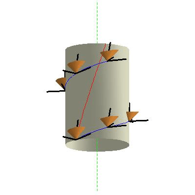
Each integral curve of the timelike unit vector field ${\vec {p}}_{0}$ appears in the cylindrical chart as a helix with constant radius (such as the red curve in the figure at right). Suppose we choose one Langevin observer and consider the other observers who ride on a ring of radius R which is rigidly rotating with angular velocity ω. Then if we take an integral curve (blue helical curve in the figure at right) of the spacelike basis vector ${\vec {p}}_{3}$ , we obtain a curve which we might hope can be interpreted as a "line of simultaneity" for the ring-riding observers. But as we see from the figure, ideal clocks carried by these ring-riding observers cannot be synchronized. This is our first hint that it is not as easy as one might expect to define a satisfactory notion of spatial geometry even for a rotating ring, much less a rotating disk!

Computing the kinematic decomposition of the Langevin congruence, we find that the acceleration vector is

\nabla _{{{\vec {p}}_{0}}}{\vec {p}}_{0}={\frac {-\omega ^{2}\,R}{1-\omega ^{2}\,R^{2}}}\;{\vec {p}}_{2}

This points radially inward and it depends only on the (constant) radius of each helical world line. The expansion tensor vanishes identically, which means that nearby Langevin observers maintain constant distance from each other. The vorticity vector is

{\vec {\Omega }}={\frac {\omega }{1-\omega ^{2}\,R^{2}}}\;{\vec {p}}_{1}

which is parallel to the axis of symmetry. This means that the world lines of the nearest neighbors of each Langevin observer are twisting about its own world line, as suggested by the figure at right. This is a kind of local notion of "swirling" or vorticity.

In contrast, note that projecting the helices onto any one of the spatial hyperslices $T=T_0$ orthogonal to the world lines of the static observers gives a circle, which is of course a closed curve. Even better, the coordinate basis vector $\partial _{\Phi }$ is a spacelike Killing vector field whose integral curves are closed spacelike curves (circles, in fact), which moreover degenerate to zero length closed curves on the axis R = 0. This expresses the fact that our spacetime exhibits cylindrical symmetry, and also exhibits a kind of global notion of the rotation of our Langevin observers.

In the figure, the magenta curve shows how the spatial vectors ${\vec {p}}_{2},\;{\vec {p}}_{3}$ are spinning about ${\vec {p}}_{1}$ (which is suppressed in the figure since the Z coordinate is inessential). That is, the vectors ${\vec {p}}_{2},\;{\vec {p}}_{3}$ are not Fermi–Walker transported along the world line, so the Langevin frame is spinning as well as non-inertial. In other words, in our straightforward derivation of the Langevin frame, we kept the frame aligned with the radial coordinate basis vector $\partial _{R}$ . By introducing a constant rate rotation of the frame carried by each Langevin observer about ${\vec {p}}_{1}$ , we could, if we wished "despin" our frame to obtain a gyrostabilized version.

Transforming to the Born chart

To obtain the Born chart, we straighten out the helical world lines of the Langevin observers using the simple coordinate transformation

t=T,\;\;z=Z,\;\;r=R,\;\;\phi =\Phi -\omega \,T

The new line element is

ds^{2}=-\left(1-\omega ^{2}\,r^{2}\right)\,dt^{2}+2\,\omega \,r^{2}\,dt\,d\phi +dz^{2}+dr^{2}+r^{2}\,d\phi ^{2}

-\infty <t,\,z<\infty ,0<r<{\frac {1}{\omega }},\;-\pi <\phi <\pi

Notice the "cross-terms" involving $dt\,d\phi$ , which show that the Born chart is not an orthogonal coordinate chart. The Born coordinates are also sometimes referred to as rotating cylindrical coordinates.

In the new chart, the world lines of the Langevin observers appear as vertical straight lines. Indeed, we can easily transform the four vector fields making up the Langevin frame into the new chart. We obtain

{\vec {p}}_{0}={\frac {1}{{\sqrt {1-\omega ^{2}\,r^{2}}}}}\,\partial _{t}

{\vec {p}}_{1}=\partial _{z},\;\;{\vec {p}}_{2}=\partial _{r}

{\vec {p}}_{3}={\frac {{\sqrt {1-\omega ^{2}\,r^{2}}}}{r}}\,\partial _{\phi }+{\frac {\omega \,r}{{\sqrt {1-\omega ^{2}\,r^{2}}}}}\,\partial _{t}

These are exactly the same vector fields as before--- they are now simply represented in a different coordinate chart!

Needless to say, in the process of "unwinding" the world lines of the Langevin observers, which appear as helices in the cylindrical chart, we "wound up" the world lines of the static observers, which now appear as helices in the Born chart! Note too that, like the Langevin frame, the Born chart is only defined on the region 0 < r < 1/ω.

If we recompute the kinematic decomposition of the Langevin observers, that is of the timelike congruence ${\vec {p}}_{0}={\frac {1}{{\sqrt {1-\omega ^{2}\,r^{2}}}}}\,\partial _{t}$ , we will of course obtain the same answer that we did before, only expressed in terms of the new chart. Specifically, the acceleration vector is

\nabla _{{{\vec {p}}_{0}}}\,{\vec {p}}_{0}={\frac {-\omega ^{2}\,r}{1-\omega ^{2}\,r^{2}}}\,{\vec {p}}_{2}

the expansion tensor vanishes, and the vorticity vector is

{\vec {\Omega }}={\frac {\omega }{1-\omega ^{2}\,r^{2}}}\;{\vec {p}}_{1}

The dual covector field of the timelike unit vector field in any frame field represents infinitesimal spatial hyperslices. However, the Frobenius integrability theorem gives a strong restriction on whether or not these spatial hyperplane elements can be "knit together" to form a family of spatial hypersurfaces which are everywhere orthogonal to the world lines of the congruence. Indeed, it turns out that this is possible, in which case we say the congruence is hypersurface orthogonal, if and only if the vorticity vector vanishes identically. Thus, while the static observers in the cylindrical chart admits a unique family of orthogonal hyperslices $T=T_0$ , the Langevin observers admit no such hyperslices. In particular, the spatial surfaces $t=t_0$ in the Born chart are orthogonal to the static observers, not to the Langevin observers. This is our second (and much more pointed) indication that defining "the spatial geometry of a rotating disk" is not as simple as one might expect.

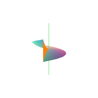
To better understand this crucial point, consider integral curves of the third Langevin frame vector

{\vec {p}}_{3}={\sqrt {1-\omega ^{2}\,r^{2}}}\,{\frac {1}{r}}\,\partial _{\phi }+{\frac {\omega \,r}{{\sqrt {1-\omega ^{2}\,r^{2}}}}}\,\partial _{t}

which pass through the radius $\phi =0,\,t=0$ . (For convenience, we will suppress the inessential coordinate z from our discussion.) These curves lie in the surface

\phi +\omega \,t-{\frac {t}{\omega \,r^{2}}}=0,\;\;-\pi <\phi <\pi

shown in the figure. We would like to regard this as a "space at a time" for our Langevin observers. But two things go wrong.

First, the Frobenius theorem tells us that ${\vec {p}}_{2},\,{\vec {p}}_{3}$ are tangent to no spatial hyperslice whatever. Indeed, except on the initial radius, the vectors ${\vec {p}}_{2}$ do not lie in our slice. Thus, while we found a spatial hypersurface, it is orthogonal to the world lines of only some our Langevin observers. Because the obstruction from the Frobenius theorem can be understood in terms of the failure of the vector fields ${\vec {p}}_{2},\,{\vec {p}}_{3}$ to form a Lie algebra, this obstruction is differential, in fact Lie theoretic. That is, it is a kind of infinitesimal obstruction to the existence of a satisfactory notion of spatial hyperslices for our rotating observers.

Second, as the figure shows, our attempted hyperslice would lead to a discontinuous notion of "time" due to the "jumps" in the integral curves (shown as a coral colored discontinuity). Alternatively, we could try to use a multivalued time. Neither of these alternatives seems very attractive! This is evidently a global obstruction. It is of course a consequence of our inability to synchronize the clocks of the Langevin observers riding even a single ring---say the rim of a disk--- much less an entire disk.

The Sagnac effect

Imagine that we have fastened a fiber-optic cable around the circumference of a ring which is rotating with steady angular velocity ω. We wish to compute the round trip travel time, as measured by a ring-riding observer, for a laser pulse sent clockwise and counterclockwise around the cable. For simplicity, we will ignore the fact that light travels through a fiber optic cable at somewhat less than the speed of light in a vacuum, and will pretend that the world line of our laser pulse is a null curve (but certainly not a null geodesic!).

In the Born line element, let us put $ds=dz=dr=0$ . This gives

(1-\omega ^{2}\,r_{0}^{2})\,dt^{2}=2\omega \,r_{0}^{2}\,dt\,d\phi +r_{0}^{2}\,d\phi ^{2}

dt={\frac {r_{0}\,d\phi }{1\pm \omega \,r_{0}}}

We obtain for the round trip travel time

\Delta t_{+}={\frac {2\pi r_{0}}{1+\omega \,r_{0}}},\;\;\Delta t_{-}={\frac {2\pi r_{0}}{1-\omega \,r_{0}}}

Putting $\delta ={\frac {\Delta t_{+}-\Delta t_{-}}{2\,\pi \,r}}$ , we find $\omega ={\frac {-1+{\sqrt {1+\delta ^{2}}}}{\delta \,r}}$ so that the ring-riding observers can determine the angular velocity of the ring (as measured by a static observer) from the difference between clockwise and counterclockwise travel times. This is known as the Sagnac effect. It is evidently a global effect.

Null Geodesics

We wish to compare the appearance of null geodesics in the cylindrical chart and the Born chart.

In the cylindrical chart, the geodesic equations read

{\ddot {T}}=0,\;\;{\ddot {Z}}=0,\;\;{\ddot {R}}-R\,{\dot {\Phi }}^{2}=0,\;\;{\ddot {\Phi }}+{\frac {2}{R}}\,{\dot {\Phi }}\,{\dot {R}}=0.

We immediately obtain the first integrals

{\dot {T}}=E,\;\;{\dot {Z}}=P,\;\;{\dot {\Phi }}={\frac {L}{R^{2}}}.

Plugging these into the expression obtained from the line element by setting $\mathrm {d} s^{2}=0$ , we obtain

{\dot {R}}^{2}=E^{2}-P^{2}-{\frac {L^{2}}{R^{2}}}\geq 0

from which we see that the minimal radius of a null geodesic is given by

E^{2}-P^{2}-{\frac {L^{2}}{R_{0}^{2}}}=0\quad

i.e.,

\quad R_{0}={\frac {L}{\sqrt {E^{2}-P^{2}}}}

hence

{\dot {R}}^{2}=L^{2}\left({\frac {1}{R_{0}^{2}}}-{\frac {1}{R^{2}}}\right).

We can now solve to obtain the null geodesics as curves parameterized by an affine parameter, as follows:

R={\sqrt {(E^{2}-P^{2})\,s^{2}+L^{2}/(E^{2}-P^{2})}}={\sqrt {(E^{2}-P^{2})\,s^{2}+R_{0}^{2}}},

T=T_{0}+E\,s,

Z=Z_{0}+P\,s,

\Phi =\Phi _{0}+\operatorname {arctan} \left({\frac {E^{2}-P^{2}}{L}}\,s\right)=\Phi _{0}+\operatorname {arctan} \left({\frac {\sqrt {E^{2}-P^{2}}}{R_{0}}}\,s\right).

More useful for our purposes is the observation that the trajectory of a null geodesic (its projection into any spatial hyperslice $T=T_0$ ) is of course a straight line, given by

R=R_{0}\,\sec(\Phi -\Phi _{0}).

To obtain the minimal radius of the line through two points (on the same side of the point of closest approach to the origin), we solve

R_{1}=R_{0}\,\sec(\Phi _{1}-\Phi _{0}),\;\;R_{2}=R_{0}\,\sec(\Phi _{2}-\Phi _{0})

which gives

R_{0}={\frac {R_{1}\,R_{2}\,|\sin(\Phi _{2}-\Phi _{1})|}{\sqrt {R_{1}^{2}-2\,R_{1}\,R_{2}\,\cos(\Phi _{2}-\Phi _{1})+R_{2}^{2}}}}.

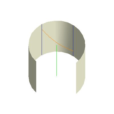
Now consider the simplest case, the radial null geodesics. An outward bound radial null geodesic may be written in the form

T=s,\;Z=Z_{0},\;R=s,

\Phi =\Phi _{0}=\omega \,R_{\mathrm {rim} }.

Transforming to the Born chart, we find that the trajectory can be written as

r=r_{\mathrm {rim} }-{\frac {\phi }{\omega }}.

Similarly for inward bound radial null geodesics. The tracks turn out to appear slightly bent in the Born chart (see figure at right). (We will see in a later section that in the Born chart, we cannot properly refer to these "tracks" as "projections", however.)

Notice that, just as a duck hunter would expect, to send a laser pulse toward the stationary observer at R = 0, the Langevin observers have to aim slightly ahead to correct for their own motion. Turning things around, to send a laser pulse toward a Langevin observer riding a counterclockwise rotating ring, the central observer has to aim, not at this observer's current position, but at the position at which he will arrive just in time to intercept the signal. These families of inward and outward bound radial null geodesics represent very different curves in spacetime, but their projections do agree.

Similarly, null geodesics between ring-riding Langevin observers appear slightly bent inward in the Born chart. To see this, write the equation of a null geodesic in the cylindrical chart in the form

T=R_{0}\,\tan(\Phi )

R=R_{0}\,\sec(\Phi )

Transforming to Born coordinates, we obtain the equations

t=r_{0}\,\tan(\phi +\omega \,t)

r=r_{0}\,\sec(\phi +\omega \,t)

Eliminating φ gives

r={\sqrt {r_{0}^{2}+t^{2}}}

which shows that the geodesic does indeed appear to bend inward. We also find that

\phi =-\omega \,{\sqrt {r^{2}-r_{0}^{2}}}+\operatorname {arctan}(t/r_{0})

This completes the description of the appearance of null geodesics in the Born chart, since every null geodesic is either radial or else has some point of closest approach to the axis of cylindrical symmetry.

Note (see figure) that a ring-riding observer trying to send a laser pulse to another ring-riding observer must aim slightly ahead of his angular coordinate as given in the Born chart, in order to compensate for the rotational motion of the target. Note too that the picture presented here is fully compatible with our expectation (see appearance of the night sky) that a moving observer will see the apparent position of other objects on his celestial sphere to be displaced toward the direction of his motion.

Radar distance in the large

Even in flat spacetime, it turns out that accelerating observers (even linearly accelerating observers; see Rindler coordinates) can employ various distinct but operationally significant notions of distance. Perhaps the simplest of these is radar distance.

Consider how a static observer at R=0 might determine his distance to a ring riding observer at R = R₀. At event C he sends a radar pulse toward the ring, which strikes the world line of a ring-riding observer at A′ and then returns to the central observer at event C″. (See the right hand diagram in the figure at right.) He then divides the elapsed time (as measured by an ideal clock he carries) by two. It is not hard to see that he obtains for this distance simply R₀ (in the cylindrical chart), or r₀ (in the Born chart).

Similarly, a ring-riding observer can determine his distance to the central observer by sending a radar pulse, at event A toward the central observer, which strikes his world line at event C′ and returns to the ring-riding observer at event A″. (See the left hand diagram in the figure at right.) It is not hard to see that he obtains for this distance $R_{0}{\sqrt {1-\omega ^{2}\,R_{0}^{2}}}$ (in the cylindrical chart) or $r_{0}{\sqrt {1-\omega ^{2}\,r_{0}^{2}}}$ (in the Born chart), a result which is somewhat smaller than the one obtained by the central observer. This is a consequence of time dilation: the elapsed time for a ring riding observer is smaller by the factor ${\sqrt {1-\omega ^{2}\,r_{0}^{2}}}$ than the time for the central observer. Thus, while radar distance has a simple operational significance, it is not even symmetric.

Just to drive home this crucial point, let us compare the radar distances obtained by two ring-riding observers with radial coordinate R = R₀. In the left hand diagram at the figure to the left, we can write the coordinates of event A as

T=0,\;Z=0,\;X=R_{0},Y=0

and we can write the coordinates of event B′ as

T=2\,R_{0}\,\sin \left({\frac {\Phi }{2}}\right),\;Z=0,

X=R_{0}\cos(\Phi ),\;Y=R_{0}\sin(\Phi )

Writing the unknown elapsed proper time as $\Delta s$ , we now write the coordinates of event A″ as

T={\frac {\Delta s}{{\sqrt {1-\omega ^{2}\,R_{0}^{2}}}}},\;Z=0

X=R_{0}\cos \left({\frac {\omega \,\Delta s}{{\sqrt {1-\omega ^{2}\,R_{0}^{2}}}}}\right),\;Y=R_{0}\sin \left({\frac {\omega \,\Delta s}{{\sqrt {1-\omega ^{2}\,R_{0}^{2}}}}}\right)

By requiring that the line segments connecting these events be null, we obtain an equation which in principle we can solve for Δ s. It turns out that this procedure gives a rather complicated nonlinear equation, so we simply present some representative numerical results. With R₀ = 1, Φ = π/2, and ω = 1/10, we find that the radar distance from A to B is about 1.308, while the distance from B to A is about 1.505. As ω tends to zero, both results tend toward $\sqrt{2} \approx 1.414$ .

Despite these possibly discouraging discrepancies, it is by no means impossible to devise a coordinate chart which is adapted to describing the physical experience of a single Langevin observer, or even a single arbitrarily accelerating observer in Minkowski spacetime. Pauri and Vallisneri have adapted the Märzke-Wheeler clock synchronization procedure to devise adapted coordinates they call Märzke-Wheeler coordinates (see the paper cited below). In the case of steady circular motion, this chart is in fact very closely related to the notion of radar distance "in the large" from a given Langevin observer.

Radar distance in the small

As was mentioned above, for various reasons the family of Langevin observers admits no family of orthogonal hyperslices. Therefore, these observers simply cannot be associated with any slicing of spacetime into a family of successive "constant time slices".

However, because the Langevin congruence is stationary, we can imagine replacing each world line in this congruence by a point. That is, we can consider the quotient space of Minkowski spacetime (or rather, the region 0 < R < 1/ω) by the Langevin congruence, which is a three-dimensional topological manifold. Even better, we can place a Riemannian metric on this quotient manifold, turning it into a three-dimensional Riemannian manifold, in such a way that the metric has a simple operational significance.

To see this, consider the Born line element

ds^{2}=-(1-\omega ^{2}\,r^{2})\,dt^{2}+2\,\omega \,r^{2}\,dt\,d\phi +dz^{2}+dr^{2}+r^{2}\,d\phi ^{2}

-\infty <t,z<\infty ,\;\;0<r<{\frac {1}{\omega }},\;\;-\pi <\phi <\pi

Setting ds² = 0 and solving for dt we obtain

dt_{+}={\frac {-\omega \,r^{2}+{\sqrt {(1-\omega ^{2}\,r^{2})\;(dz^{2}+dr^{2})+r^{2}\,d\phi ^{2}}}}{1-\omega ^{2}\,r^{2}}}

dt_{-}={\frac {-\omega \,r^{2}-{\sqrt {(1-\omega ^{2}\,r^{2})\;(dz^{2}+dr^{2})+r^{2}\,d\phi ^{2}}}}{1-\omega ^{2}\,r^{2}}}

The elapsed proper time for a roundtrip radar blip emitted by a Langevin observer is then

{\sqrt {1-\omega ^{2}\,r^{2}}}\;{\frac {dt_{+}-dt_{-}}{2}}={\sqrt {dz^{2}+dr^{2}+{\frac {r^{2}\,d\phi ^{2}}{1-\omega ^{2}\,r^{2}}}}}

Therefore, in our quotient manifold, the Riemannian line element

d\sigma ^{2}=dz^{2}+dr^{2}+{\frac {r^{2}\,d\phi ^{2}}{1-\omega ^{2}\,r^{2}}}

-\infty <t<\infty ,\;\;0<r<{\frac {1}{\omega }},\;\;-\pi <\phi <\pi

corresponds to distance between infinitesimally nearby Langevin observers. We will call it the Langevin-Landau-Lifschitz metric, and we can call this notion of distance radar distance "in the small".

This metric was first given by Langevin, but the interpretation in terms of radar distance "in the small" is due to Lev Landau and Evgeny Lifshitz, who generalized the construction to work for the quotient of any Lorentzian manifold by a stationary timelike congruence.

If we adopt the coframe

\theta ^{{\hat {1}}}=dz,\;\;\theta ^{{\hat {2}}}=dr,\;\;\theta ^{{\hat {3}}}={\frac {r\,d\phi }{{\sqrt {1-\omega ^{2}\,r^{2}}}}}

we can easily compute the Riemannian curvature tensor of our three-dimensional quotient manifold. It has only one independent nontrivial component,

{R^{{{\hat {2}}}}}_{{{\hat {3}}{\hat {2}}{\hat {3}}}}={\frac {-3\,\omega ^{2}}{(1-\omega ^{2}r^{2})^{2}}}=-3\,\omega ^{2}\;\left(1+2\,\omega ^{2}\,r^{2}\right)+O(\omega ^{6}\,r^{6})

Thus, in some sense, the geometry of a rotating disk is curved, as Theodor Kaluza claimed (without proof) as early as 1910. In fact, to fourth order in ω it has the geometry of the hyperbolic plane, just as Kaluza claimed.

Warning: as we have seen, there are many possible notions of distance which can be employed by Langevin observers riding on a rigidly rotating disk, so statements referring to "the geometry of a rotating disk" always require careful qualification.

To drive home this important point, let us use the Landau-Lifschitz metric to compute the distance between a Langevin observer riding a ring with radius R₀ and a central static observer. To do this, we need only integrate our line element over the appropriate null geodesic track. From our earlier work, we see that we must plug

dr={\frac {d\phi }{\omega }}

into our line element and integrate. This gives

\Delta =\int _{{r_{0}}}^{0}{\frac {dr}{{\sqrt {1-\omega ^{2}\,r^{2}}}}}={\frac {\arcsin(\omega r_{0})}{\omega }}=r_{0}+{\frac {\omega ^{2}\,r_{0}^{3}}{6}}+O(r_{0}^{4})

Because we are now dealing with a Riemannian metric, this notion of distance is of course symmetric under interchanging the two observers, unlike radar distance "in the large". The values given by this notion are intermediate between the radar distances computed in the previous section. For example, for r₀ = 1, ω = 1/2, we find approximately Δ = 1.047, which can be compared with 1.155 for the distance from the ring-riding observer to the central observer, or 1 for the central observer to the ring-riding observer. Also, because up to second order the Landau-Lifschitz metric agrees with radar distance "in the large", we see that the curvature tensor we just computed does have operational significance: while radar distance "in the large" between pairs of Langevin observers is certainly not a Riemannian notion of distance, the distance between pairs of nearby Langevin observers does correspond to a Riemannian distance, given by the Langevin-Landau-Lifschitz metric. (In the felicitous phrase of Howard Percy Robertson, this is kinematics im kleinem.)

One way to see that all reasonable notions of spatial distance for our Langevin observers agree for nearby observers is to show, following Nathan Rosen, that for any one Langevin observer, an instantaneously comoving inertial observer will also obtain the distances given by the Langevin-Landau-Lifschitz metric, for very small distances.

Summary

Observers riding on a rigidly rotating disk will conclude from measurements of small distances between themselves that the geometry of the disk is non-Euclidean. Regardless of which method they use, they will conclude that the geometry is well approximated by a certain Riemannian metric, namely the Langevin-Landau-Lifschitz metric. This is in turn very well approximated by the geometry of the hyperbolic plane (with the constant negative curvature -3 ω²). But if these observers measure larger distances, they will obtain different results, depending upon which method of measurement they use! In all such cases, however, they will most likely obtain results which are inconsistent with any Riemannian metric. In particular, if they use the simplest notion of distance, radar distance, owing to various effects such as the asymmetry already noted, they will conclude that the "geometry" of the disk is not only non-Euclidean, it is non-Riemannian.

References

A few papers of historical interest:

Born, M. (1909). "Die Theorie des starren Elektrons in der Kinematik des Relativitäts-Prinzipes". Ann. Phys. 30: 1. Bibcode:1909AnP...335....1B. doi:10.1002/andp.19093351102.
- Wikisource translation: The Theory of the Rigid Electron in the Kinematics of the Principle of Relativity
Ehrenfest, P. (1909). "Gleichförmige Rotation starrer Körper und Relativitätstheorie". Phys. Zeitschrift. 10: 918.
- Wikisource translation: Uniform Rotation of Rigid Bodies and the Theory of Relativity
Langevin, P. (1935). "Remarques au sujet de la Note de Prunier". C. R. Acad. Sci. Paris. 200: 48.

A few classic references:

Grøn, Ø. (1975). "Relativistic description of a rotating disk". Amer. J. Phys. 43 (10): 869–876. Bibcode:1975AmJPh..43..869G. doi:10.1119/1.9969.
Landau, L. D. & Lifschitz, E. M. (1980). The Classical Theory of Fields (4th ed.). London: Butterworth-Heinemann. ISBN 0-7506-2768-9. See Section 84 for the Landau-Lifschitz metric on the quotient of a Lorentzian manifold by a stationary congruence; see the problem at the end of Section 89 for the application to Langevin observers.

Selected recent sources:

Rizzi, G. & Ruggiero, M. L. (2004). Relativity in Rotating Frames. Dordrecht: Kluwer. ISBN 1-4020-1805-3. This book contains a valuable historical survey by Øyvind Grøn and some other papers on the Ehrenfest paradox and related controversies and a paper by Lluis Bel discussing the Langevin congruence. Hundreds of additional references may be found in this book.
Pauri, Massimo & Vallisneri, Michele (2000). "Märzke-Wheeler coordinates for accelerated observers in special relativity". Found. Phys. Lett. 13 (5): 401–425. doi:10.1023/A:1007861914639. Studies a coordinate chart constructed using radar distance "in the large" from a single Langevin observer. See also the eprint version.

External links

The Rigid Rotating Disk in Relativity, by Michael Weiss (1995), from the sci.physics FAQ.

This article is issued from Wikipedia - version of the 12/3/2016. The text is available under the Creative Commons Attribution/Share Alike but additional terms may apply for the media files.