Binary space partitioning
In computer science, binary space partitioning (BSP) is a method for recursively subdividing a space into convex sets by hyperplanes. This subdivision gives rise to a representation of objects within the space by means of a tree data structure known as a BSP tree.
Binary space partitioning was developed in the context of 3D computer graphics,[1][2] where the structure of a BSP tree allows spatial information about the objects in a scene that is useful in rendering, such as their ordering from front-to-back with respect to a viewer at a given location, to be accessed rapidly. Other applications include performing geometrical operations with shapes (constructive solid geometry) in CAD,[3] collision detection in robotics and 3-D video games, ray tracing and other computer applications that involve handling of complex spatial scenes.
Overview
Binary space partitioning is a generic process of recursively dividing a scene into two until the partitioning satisfies one or more requirements. It can be seen as a generalisation of other spatial tree structures such as k-d trees and quadtrees, one where hyperplanes that partition the space may have any orientation, rather than being aligned with the coordinate axes as they are in k-d trees or quadtrees. When used in computer graphics to render scenes composed of planar polygons, the partitioning planes are frequently (but not always) chosen to coincide with the planes defined by polygons in the scene.
The specific choice of partitioning plane and criterion for terminating the partitioning process varies depending on the purpose of the BSP tree. For example, in computer graphics rendering, the scene is divided until each node of the BSP tree contains only polygons that can render in arbitrary order. When back-face culling is used, each node therefore contains a convex set of polygons, whereas when rendering double-sided polygons, each node of the BSP tree contains only polygons in a single plane. In collision detection or ray tracing, a scene may be divided up into primitives on which collision or ray intersection tests are straightforward.
Binary space partitioning arose from the computer graphics need to rapidly draw three-dimensional scenes composed of polygons. A simple way to draw such scenes is the painter's algorithm, which produces polygons in order of distance from the viewer, back to front, painting over the background and previous polygons with each closer object. This approach has two disadvantages: time required to sort polygons in back to front order, and the possibility of errors in overlapping polygons. Fuchs and co-authors[2] showed that constructing a BSP tree solved both of these problems by providing a rapid method of sorting polygons with respect to a given viewpoint (linear in the number of polygons in the scene) and by subdividing overlapping polygons to avoid errors that can occur with the painter's algorithm. A disadvantage of binary space partitioning is that generating a BSP tree can be time-consuming. Typically, it is therefore performed once on static geometry, as a pre-calculation step, prior to rendering or other realtime operations on a scene. The expense of constructing a BSP tree makes it difficult and inefficient to directly implement moving objects into a tree.
BSP trees are often used by 3D video games, particularly first-person shooters and those with indoor environments. Game engines utilising BSP trees include the Doom engine (probably the earliest game to use a BSP data structure was Doom), the Quake engine and its descendants. In video games, BSP trees containing the static geometry of a scene are often used together with a Z-buffer, to correctly merge movable objects such as doors and characters onto the background scene. While binary space partitioning provides a convenient way to store and retrieve spatial information about polygons in a scene, it does not solve the problem of visible surface determination.
Generation
The canonical use of a BSP tree is for rendering polygons (that are double-sided, that is, without back-face culling) with the painter's algorithm. Each polygon is designated with a front side and a back side which could be chosen arbitrarily and only affects the structure of the tree but not the required result.[2] Such a tree is constructed from an unsorted list of all the polygons in a scene. The recursive algorithm for construction of a BSP tree from that list of polygons is:[2]
- Choose a polygon P from the list.
- Make a node N in the BSP tree, and add P to the list of polygons at that node.
- For each other polygon in the list:
- If that polygon is wholly in front of the plane containing P, move that polygon to the list of nodes in front of P.
- If that polygon is wholly behind the plane containing P, move that polygon to the list of nodes behind P.
- If that polygon is intersected by the plane containing P, split it into two polygons and move them to the respective lists of polygons behind and in front of P.
- If that polygon lies in the plane containing P, add it to the list of polygons at node N.
- Apply this algorithm to the list of polygons in front of P.
- Apply this algorithm to the list of polygons behind P.
The following diagram illustrates the use of this algorithm in converting a list of lines or polygons into a BSP tree. At each of the eight steps (i.-viii.), the algorithm above is applied to a list of lines, and one new node is added to the tree.
| Start with a list of lines, (or in 3-D, polygons) making up the scene. In the tree diagrams, lists are denoted by rounded rectangles and nodes in the BSP tree by circles. In the spatial diagram of the lines, the direction chosen to be the 'front' of a line is denoted by an arrow. |  | |
| i. | Following the steps of the algorithm above,
|
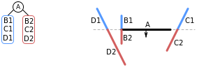 |
| ii. | We now apply the algorithm to the list of lines in front of A (containing B2, C2, D2). We choose a line, B2, add it to a node and split the rest of the list into those lines that are in front of B2 (D2), and those that are behind it (C2, D3). | 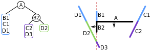 |
| iii. | Choose a line, D2, from the list of lines in front of B2. It is the only line in the list, so after adding it to a node, nothing further needs to be done. |  |
| iv. | We are done with the lines in front of B2, so consider the lines behind B2 (C2 and D3). Choose one of these (C2), add it to a node, and put the other line in the list (D3) into the list of lines in front of C2. | 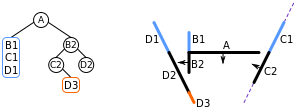 |
| v. | Now look at the list of lines in front of C2. There is only one line (D3), so add this to a node and continue. |  |
| vi. | We have now added all of the lines in front of A to the BSP tree, so we now start on the list of lines behind A. Choosing a line (B1) from this list, we add B1 to a node and split the remainder of the list into lines in front of B1 (i.e. D1), and lines behind B1 (i.e. C1). | 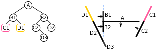 |
| vii. | Processing first the list of lines in front of B1, D1 is the only line in this list, so add this to a node and continue. | 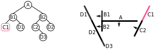 |
| viii. | Looking next at the list of lines behind B1, the only line in this list is C1, so add this to a node, and the BSP tree is complete. |  |
The final number of polygons or lines in a tree is often larger (sometimes much larger[2]) than the original list, since lines or polygons that cross the partitioning plane must be split into two. It is desirable to minimize this increase, but also to maintain reasonable balance in the final tree. The choice of which polygon or line is used as a partitioning plane (in step 1 of the algorithm) is therefore important in creating an efficient BSP tree.
Traversal
A BSP tree is traversed in a linear time, in an order determined by the particular function of the tree. Again using the example of rendering double-sided polygons using the painter's algorithm, to draw a polygon P correctly requires that all polygons behind the plane P lies in must be drawn first, then polygon P, then finally the polygons in front of P. If this drawing order is satisfied for all polygons in a scene, then the entire scene renders in the correct order. This procedure can be implemented by recursively traversing a BSP tree using the following algorithm.[2] From a given viewing location V, to render a BSP tree,
- If the current node is a leaf node, render the polygons at the current node.
- Otherwise, if the viewing location V is in front of the current node:
- Render the child BSP tree containing polygons behind the current node
- Render the polygons at the current node
- Render the child BSP tree containing polygons in front of the current node
- Otherwise, if the viewing location V is behind the current node:
- Render the child BSP tree containing polygons in front of the current node
- Render the polygons at the current node
- Render the child BSP tree containing polygons behind the current node
- Otherwise, the viewing location V must be exactly on the plane associated with the current node. Then:
- Render the child BSP tree containing polygons in front of the current node
- Render the child BSP tree containing polygons behind the current node

Applying this algorithm recursively to the BSP tree generated above results in the following steps:
- The algorithm is first applied to the root node of the tree, node A. V is in front of node A, so we apply the algorithm first to the child BSP tree containing polygons behind A
- This tree has root node B1. V is behind B1 so first we apply the algorithm to the child BSP tree containing polygons in front of B1:
- This tree is just the leaf node D1, so the polygon D1 is rendered.
- We then render the polygon B1.
- We then apply the algorithm to the child BSP tree containing polygons behind B1:
- This tree is just the leaf node C1, so the polygon C1 is rendered.
- This tree has root node B1. V is behind B1 so first we apply the algorithm to the child BSP tree containing polygons in front of B1:
- We then draw the polygons of A
- We then apply the algorithm to the child BSP tree containing polygons in front of A
- This tree has root node B2. V is behind B2 so first we apply the algorithm to the child BSP tree containing polygons in front of B2:
- This tree is just the leaf node D2, so the polygon D2 is rendered.
- We then render the polygon B2.
- We then apply the algorithm to the child BSP tree containing polygons behind B2:
- This tree has root node C2. V is in front of C2 so first we would apply the algorithm to the child BSP tree containing polygons behind C2. There is no such tree, however, so we continue.
- We render the polygon C2.
- We apply the algorithm to the child BSP tree containing polygons in front of C2
- This tree is just the leaf node D3, so the polygon D3 is rendered.
- This tree has root node B2. V is behind B2 so first we apply the algorithm to the child BSP tree containing polygons in front of B2:
The tree is traversed in linear time and renders the polygons in a far-to-near ordering (D1, B1, C1, A, D2, B2, C2, D3) suitable for the painter's algorithm.
Timeline
- 1969 Schumacker et al.[1] published a report that described how carefully positioned planes in a virtual environment could be used to accelerate polygon ordering. The technique made use of depth coherence, which states that a polygon on the far side of the plane cannot, in any way, obstruct a closer polygon. This was used in flight simulators made by GE as well as Evans and Sutherland. However, creation of the polygonal data organization was performed manually by scene designer.
- 1980 Fuchs et al.[2] extended Schumacker’s idea to the representation of 3D objects in a virtual environment by using planes that lie coincident with polygons to recursively partition the 3D space. This provided a fully automated and algorithmic generation of a hierarchical polygonal data structure known as a Binary Space Partitioning Tree (BSP Tree). The process took place as an off-line preprocessing step that was performed once per environment/object. At run-time, the view-dependent visibility ordering was generated by traversing the tree.
- 1981 Naylor's Ph.D thesis provided a full development of both BSP trees and a graph-theoretic approach using strongly connected components for pre-computing visibility, as well as the connection between the two methods. BSP trees as a dimension independent spatial search structure was emphasized, with applications to visible surface determination. The thesis also included the first empirical data demonstrating that the size of the tree and the number of new polygons was reasonable (using a model of the Space Shuttle).
- 1983 Fuchs et al. described a micro-code implementation of the BSP tree algorithm on an Ikonas frame buffer system. This was the first demonstration of real-time visible surface determination using BSP trees.
- 1987 Thibault and Naylor[3] described how arbitrary polyhedra may be represented using a BSP tree as opposed to the traditional b-rep (boundary representation). This provided a solid representation vs. a surface based-representation. Set operations on polyhedra were described using a tool, enabling Constructive Solid Geometry (CSG) in real-time. This was the fore runner of BSP level design using "brushes", introduced in the Quake editor and picked up in the Unreal Editor.
- 1990 Naylor, Amanatides, and Thibault provided an algorithm for merging two BSP trees to form a new BSP tree from the two original trees. This provides many benefits including: combining moving objects represented by BSP trees with a static environment (also represented by a BSP tree), very efficient CSG operations on polyhedra, exact collisions detection in O(log n * log n), and proper ordering of transparent surfaces contained in two interpenetrating objects (has been used for an x-ray vision effect).
- 1990 Teller and Séquin proposed the offline generation of potentially visible sets to accelerate visible surface determination in orthogonal 2D environments.
- 1991 Gordon and Chen [CHEN91] described an efficient method of performing front-to-back rendering from a BSP tree, rather than the traditional back-to-front approach. They utilised a special data structure to record, efficiently, parts of the screen that have been drawn, and those yet to be rendered. This algorithm, together with the description of BSP Trees in the standard computer graphics textbook of the day (Computer Graphics: Principles and Practice) was used by John Carmack in the making of Doom (video game).
- 1992 Teller’s PhD thesis described the efficient generation of potentially visible sets as a pre-processing step to accelerate real-time visible surface determination in arbitrary 3D polygonal environments. This was used in Quake (video game) and contributed significantly to that game's performance.
- 1993 Naylor answered the question of what characterizes a good BSP tree. He used expected case models (rather than worst case analysis) to mathematically measure the expected cost of searching a tree and used this measure to build good BSP trees. Intuitively, the tree represents an object in a multi-resolution fashion (more exactly, as a tree of approximations). Parallels with Huffman codes and probabilistic binary search trees are drawn.
- 1993 Hayder Radha's PhD thesis described (natural) image representation methods using BSP trees. This includes the development of an optimal BSP-tree construction framework for any arbitrary input image. This framework is based on a new image transform, known as the Least-Square-Error (LSE) Partitioning Line (LPE) transform. H. Radha's thesis also developed an optimal rate-distortion (RD) image compression framework and image manipulation approaches using BSP trees.
See also
- k-d tree
- Octree
- quadtree
- Hierarchical clustering, an alternative way to divide 3d model data for efficient rendering.
References
- 1 2 Schumacker, Robert A.; Brand, Brigitta; Gilliland, Maurice G.; Sharp, Werner H (1969). Study for Applying Computer-Generated Images to Visual Simulation (Report). U.S. Air Force Human Resources Laboratory. p. 142. AFHRL-TR-69-14.
- 1 2 3 4 5 6 7 Fuchs, Henry; Kedem, Zvi. M; Naylor, Bruce F. (1980). "On Visible Surface Generation by A Priori Tree Structures". SIGGRAPH '80 Proceedings of the 7th annual conference on Computer graphics and interactive techniques. ACM, New York. pp. 124–133. doi:10.1145/965105.807481.
- 1 2 Thibault, William C.; Naylor, Bruce F. (1987). "Set operations on polyhedra using binary space partitioning trees". SIGGRAPH '87 Proceedings of the 14th annual conference on Computer graphics and interactive techniques. ACM, New York. pp. 153–162. doi:10.1145/37402.37421.
Additional references
- [NAYLOR90] B. Naylor, J. Amanatides, and W. Thibualt, "Merging BSP Trees Yields Polyhedral Set Operations", Computer Graphics (Siggraph '90), 24(3), 1990.
- [NAYLOR93] B. Naylor, "Constructing Good Partitioning Trees", Graphics Interface (annual Canadian CG conference) May, 1993.
- [CHEN91] S. Chen and D. Gordon. “Front-to-Back Display of BSP Trees.” IEEE Computer Graphics & Algorithms, pp 79–85. September 1991.
- [RADHA91] H. Radha, R. Leoonardi, M. Vetterli, and B. Naylor “Binary Space Partitioning Tree Representation of Images,” Journal of Visual Communications and Image Processing 1991, vol. 2(3).
- [RADHA93] H. Radha, "Efficient Image Representation using Binary Space Partitioning Trees.", Ph.D. Thesis, Columbia University, 1993.
- [RADHA96] H. Radha, M. Vetterli, and R. Leoonardi, “Image Compression Using Binary Space Partitioning Trees,” IEEE Transactions on Image Processing, vol. 5, No.12, December 1996, pp. 1610–1624.
- [WINTER99] AN INVESTIGATION INTO REAL-TIME 3D POLYGON RENDERING USING BSP TREES. Andrew Steven Winter. April 1999. available online
- Mark de Berg; Marc van Kreveld; Mark Overmars & Otfried Schwarzkopf (2000). Computational Geometry (2nd revised ed.). Springer-Verlag. ISBN 3-540-65620-0. Section 12: Binary Space Partitions: pp. 251–265. Describes a randomized Painter's Algorithm.
- Christer Ericson: Real-Time Collision Detection (The Morgan Kaufmann Series in Interactive 3-D Technology). Verlag Morgan Kaufmann, S. 349-382, Jahr 2005, ISBN 1-55860-732-3
External links
- BSP trees presentation
- Another BSP trees presentation
- A Java applet that demonstrates the process of tree generation
- A Master Thesis about BSP generating
- BSP Trees: Theory and Implementation
- BSP in 3D space